Business Mathematics MTH367 Lecture 1 Instructor Dr Muhammad
Business Mathematics MTH-367 Lecture 1

Instructor: Dr. Muhammad Imran Qureshi Assistant Professor Department of Mathematics COMSATS Institute of Information Technology Park Road, Chak Shahzad, Islamabad Ph. D. Mathematics University of Oxford, UK
Books • Text Book: Applied Mathematics for Business, Economics, and the Social Sciences (4 th Edition); by Frank S. Budnick • Additional Reading: Introductory Mathematical Analysis for Business, Economics, and the Life and Social Sciences; by Ernest F. Haeussler, Jr. Richard S. Paul, 8 th Edition
Grading • • Credit hours (3, 0) Total marks = 100 Sessional 1 = 10 points Sessional 2 = 15 points 4 quizzes (MCQs only) 4 assignments Final Exam = 50 points
Course Objectives • Students will be able to understand business world and its associated mathematical procedures. • To provide solid mathematical preparation and foundation for students continuing their studies and their careers in the areas of accounting, marketing, retailing, banking, office administration, management, finance, insurance, real estate, computer information systems, and general business administration. • To provide an ideal learning for small business management, entrepreneurship, and personal finance applications.
Course Objectives cont’d • To enable students to use linear programming tools such as Graphical method, simplex method, and Assignment and Transportation problem to cover a large area of mathematical optimization procedures.
Course Outline • Linear Equations • System of Linear Equations and its applications in Business. • Mathematical Functions and its types • Applications of linear, quadratic and Exponential functions in Finance and Business. • Mathematics of finance.
Course Outline Cont’d • • Linear programming Graphical Method Simplex Method Special Phenomenon Dual Problem Transportation and Assignment Models Solutions to Transportation Models, Assignment Model and method of Solution
Course Outline Cont’d. . . • • Limits, Average Rate of change, Differentiation Additional Rules of Differentiation Optimization, Identification of Maxima and Minima Revenue, Cost, and Profit Applications Integration and Techniques of integration Differential Equations and its Applications Definite integral, Applications of integral Calculus. Functions of several variables, Partial Derivatives and its applications.
Chapter wise contents • Chapter 2, 3: Linear Equations and System of Linear Equations, Applications. • Chapter 4, 5, 6, 7: Mathematical Functions, Applications • Chapter 8: Mathematics of Finance
Chapter wise contents Cont’d • Chapter 10: Linear Programming • Chapter 11: The Simplex Method • Chapter 12: Transportation and Assignment Models
Course Outline Cont’d. . . THE CALCULUS • Chapter 15: Differentiation • Chapter 16: Optimization; Methodology • Chapter 17: Optimization; Applications • Chapter 18: Integral Calculus; An Introduction • Chapter 19: Integral Calculus; Applications • Chapter 20: Functions of Several Variables
Chapter 2 Linear Equations
Objectives • Provide a thorough understanding of the algebraic and graphical characteristics of linear equations • Provide the tools which allow one to determine the equation which represents a linear relationship • Illustrate some applications
Today’s Topics • • Linear Equations in two Variables Linear Equations with n Variables; Graphical Characteristics of Two Variable Equation • Slope, Formulae to Find Slope • Determining the equation of straight line
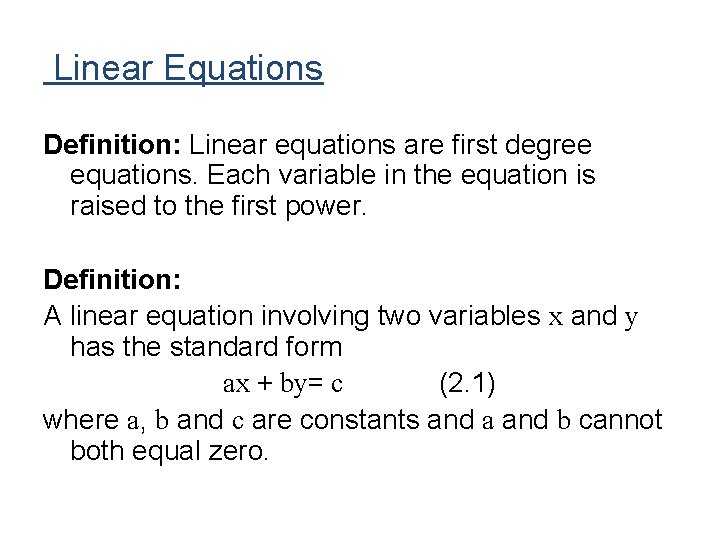
Linear Equations Definition: Linear equations are first degree equations. Each variable in the equation is raised to the first power. Definition: A linear equation involving two variables x and y has the standard form ax + by= c (2. 1) where a, b and c are constants and a and b cannot both equal zero.
Note: The presence of terms having power other than 1 or product of variables, e. g. (xy) would exclude an equation from being linear. Name of the variables may be different from x and y.
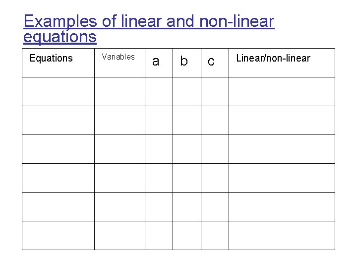
Examples of linear and non-linear equations Equations Variables a b c Linear/non-linear
Solution set of an equation Given a linear equation ax + by= c, the solution set for the equation (2. 1) is the set of all ordered pairs (x, y) which satisfy the equation. S={(x, y)|ax+by=c} For any linear equation, S consists of an infinite number of elements. Method: • Assume a value of one variable • Substitute this into the equation • Solve for the other variable
Examples 2 x + 4 y= 16 1) Determine the pair of values which satisfy the equation when x=-2 2) Determine the pair of values which satisfy the equation when y=0

Linear equation with n variables Definition A linear equation involving n variables x 1, x 2, . . . , xn has the general form a 1 x 1 + a 2 x 2+. . . + an xn = b where
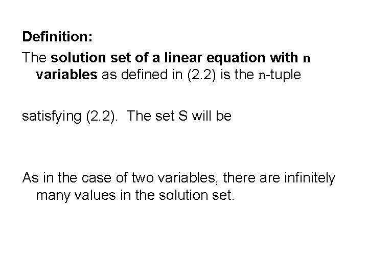
Definition: The solution set of a linear equation with n variables as defined in (2. 2) is the n-tuple satisfying (2. 2). The set S will be As in the case of two variables, there are infinitely many values in the solution set.
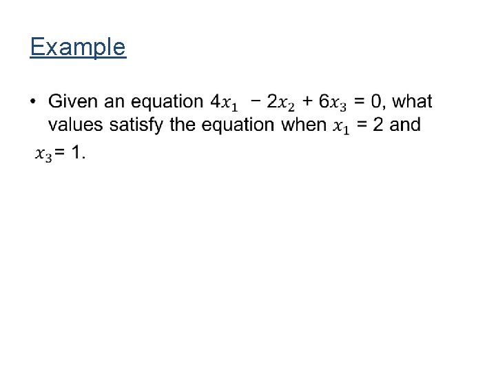
Example •
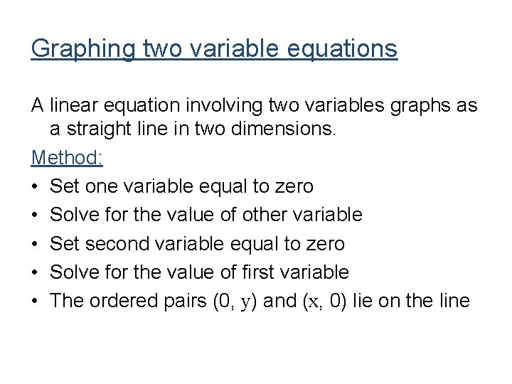
Graphing two variable equations A linear equation involving two variables graphs as a straight line in two dimensions. Method: • Set one variable equal to zero • Solve for the value of other variable • Set second variable equal to zero • Solve for the value of first variable • The ordered pairs (0, y) and (x, 0) lie on the line
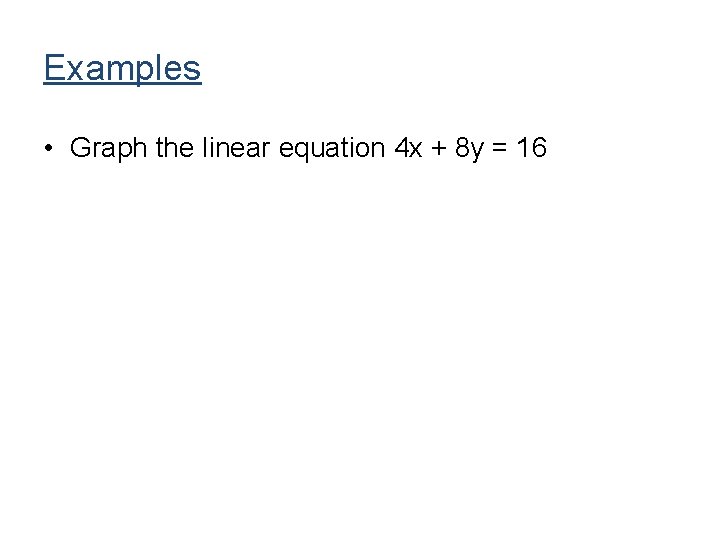
Examples • Graph the linear equation 4 x + 8 y = 16
Examples cont’d • Graph the linear equation 4 x - 7 y = 0

Intercepts x-intercept The x-intercept of an equation is the point where the graph of the equation crosses the x-axis, i. e. y=0. y-intercept The y-intercept of an equation is the point where the graph of the equation crosses the y-axis, i. e. x=0 • Equations of the form x=k has no y-intercept • Equations of the form y=k has no x-intercept
Slope • Any straight line with the exception of vertical lines can be characterized by its slope. • Slope represents the inclination of a line or equivalently it shows the rate at which the line raises and fall or how steep the line is.
Graphical explanation of slope
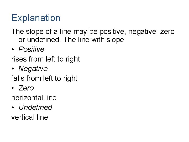
Explanation The slope of a line may be positive, negative, zero or undefined. The line with slope • Positive rises from left to right • Negative falls from left to right • Zero horizontal line • Undefined vertical line
Note: The sign of the slope represents whether the line falling or raising. It’s mag
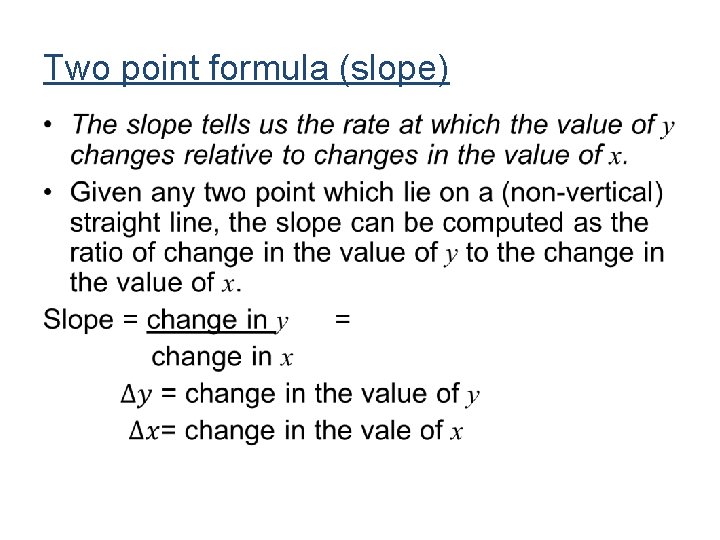
Two point formula (slope) •
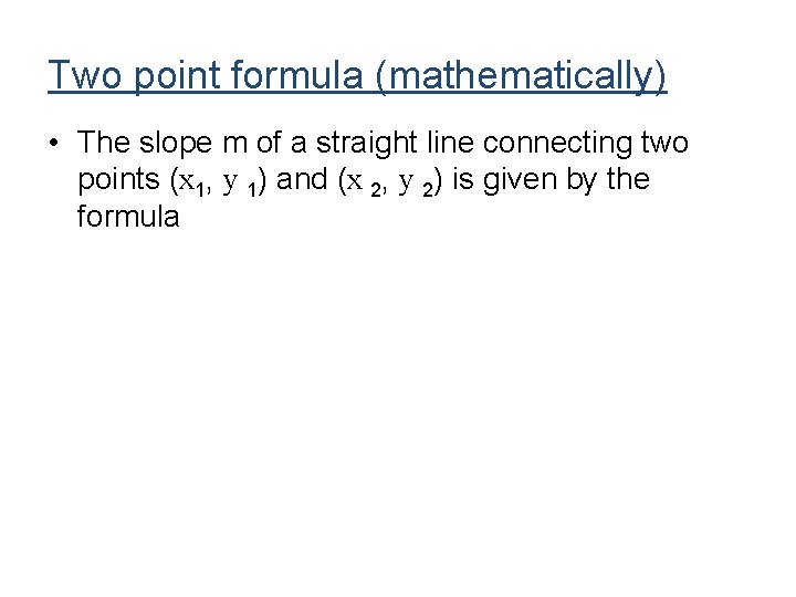
Two point formula (mathematically) • The slope m of a straight line connecting two points (x 1, y 1) and (x 2, y 2) is given by the formula
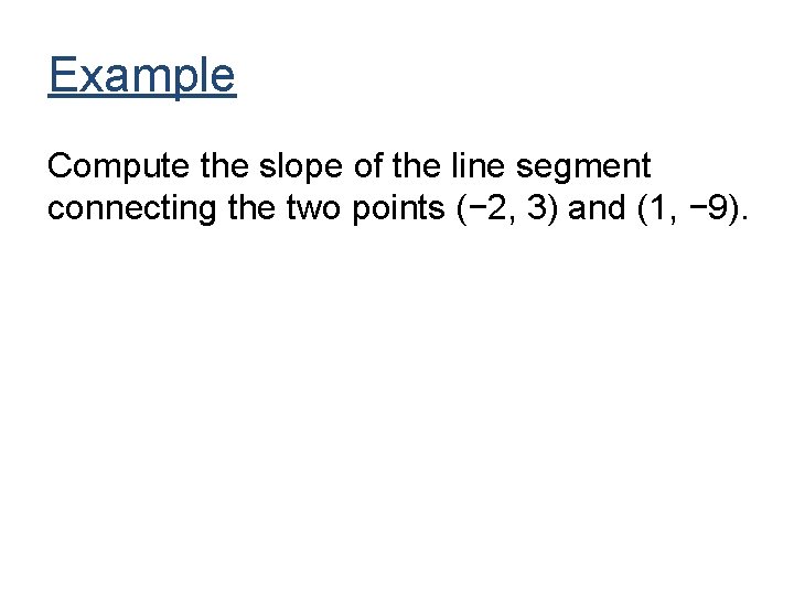
Example Compute the slope of the line segment connecting the two points (− 2, 3) and (1, − 9).
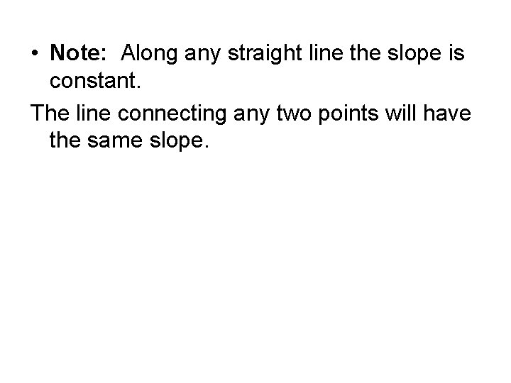
• Note: Along any straight line the slope is constant. The line connecting any two points will have the same slope.
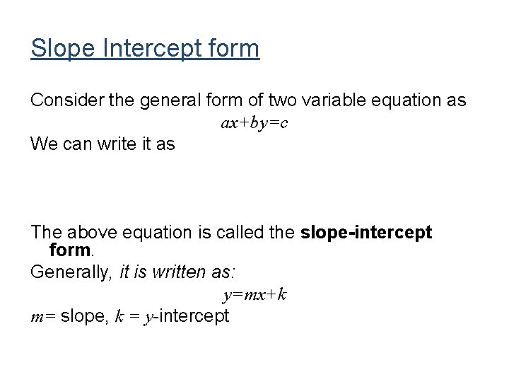
Slope Intercept form Consider the general form of two variable equation as ax+by=c We can write it as The above equation is called the slope-intercept form. Generally, it is written as: y=mx+k m= slope, k = y-intercept
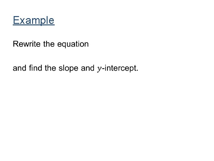
Example •
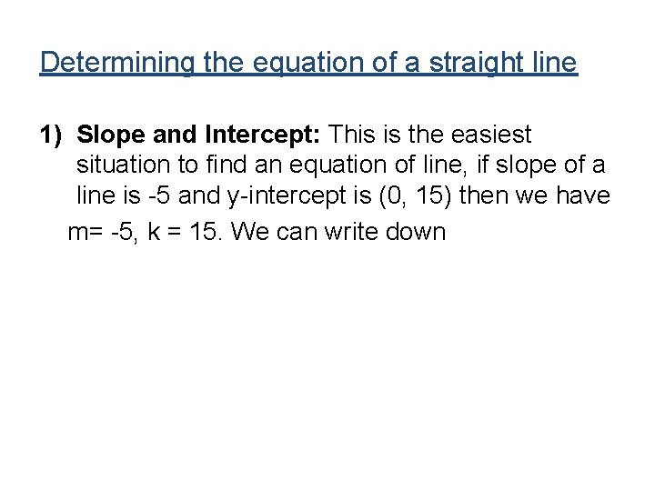
Determining the equation of a straight line 1) Slope and Intercept: This is the easiest situation to find an equation of line, if slope of a line is -5 and y-intercept is (0, 15) then we have m= -5, k = 15. We can write down
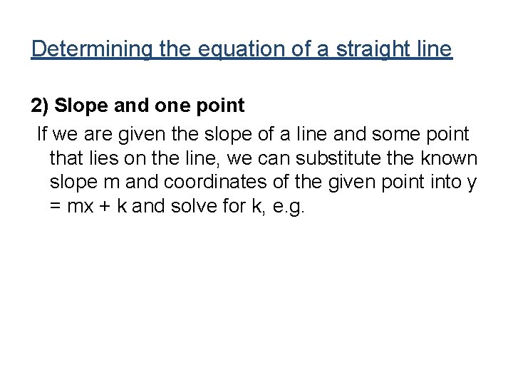
Determining the equation of a straight line 2) Slope and one point If we are given the slope of a line and some point that lies on the line, we can substitute the known slope m and coordinates of the given point into y = mx + k and solve for k, e. g.
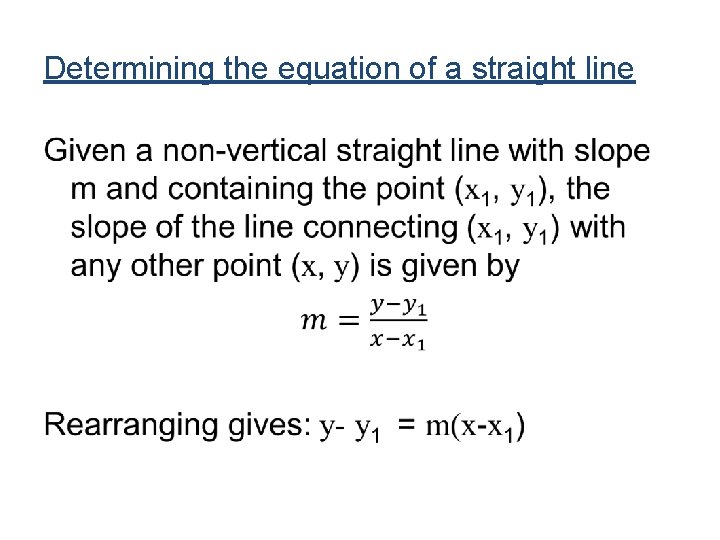
Determining the equation of a straight line •
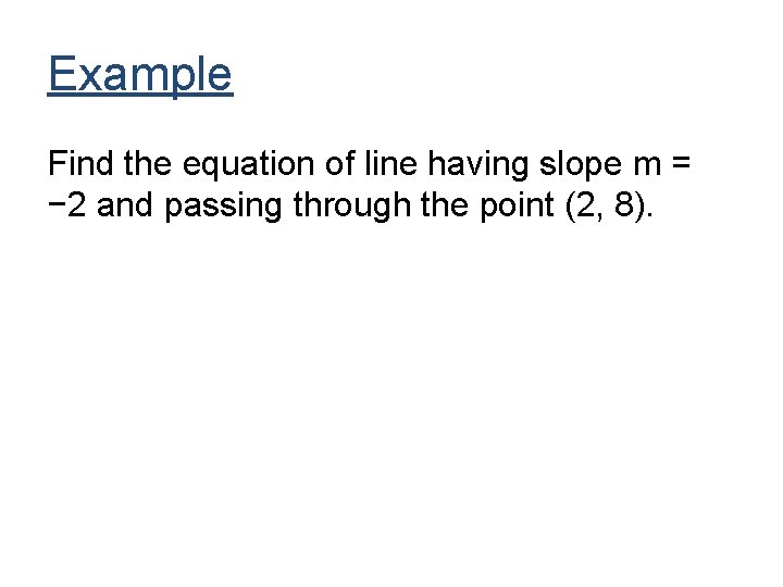
Example Find the equation of line having slope m = − 2 and passing through the point (2, 8).
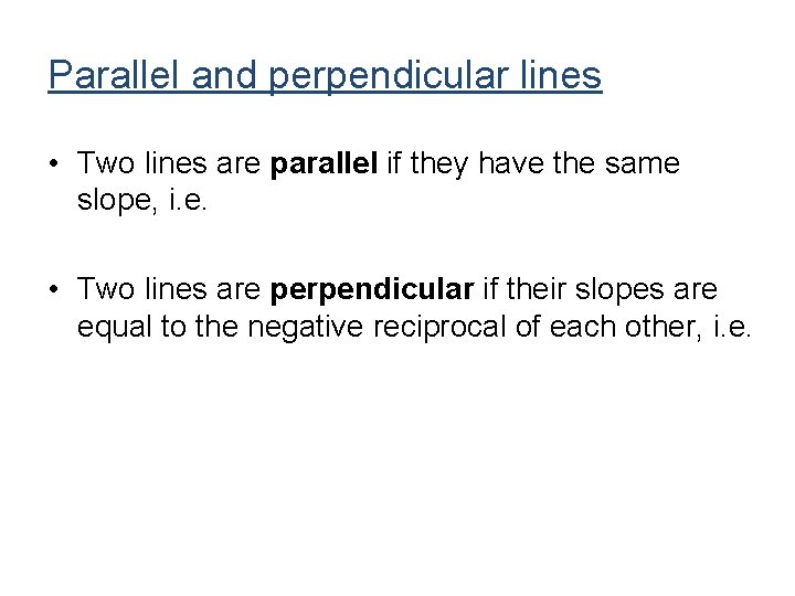
Parallel and perpendicular lines • Two lines are parallel if they have the same slope, i. e. • Two lines are perpendicular if their slopes are equal to the negative reciprocal of each other, i. e.
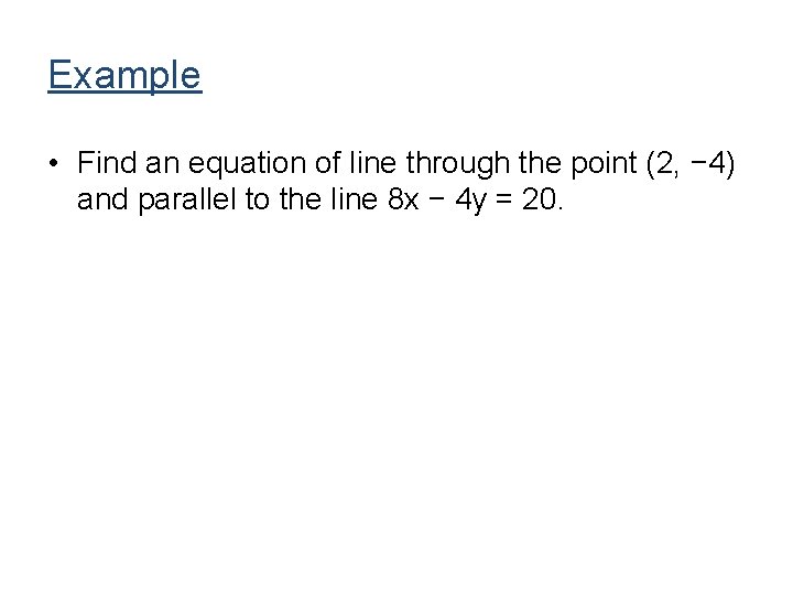
Example • Find an equation of line through the point (2, − 4) and parallel to the line 8 x − 4 y = 20.

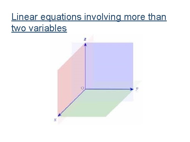
Linear equations involving more than two variables
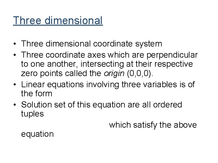
Three dimensional • Three dimensional coordinate system • Three coordinate axes which are perpendicular to one another, intersecting at their respective zero points called the origin (0, 0, 0). • Linear equations involving three variables is of the form • Solution set of this equation are all ordered tuples which satisfy the above equation
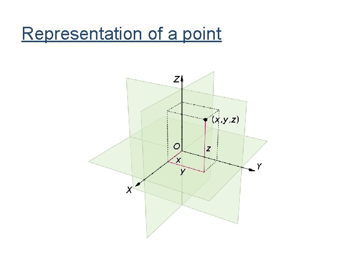
Representation of a point
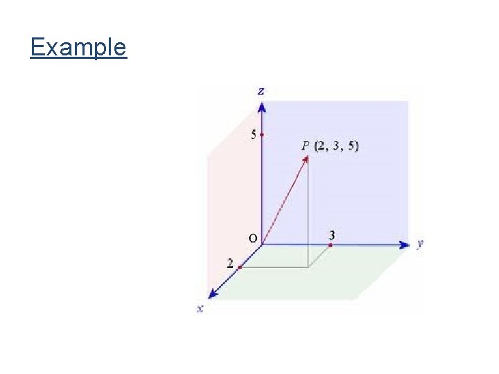
Example
Summary • • Linear Equations in two Variables Linear Equations with n Variables; Graphical Characteristics of Two Variable Equation • Slope, Formulae to Find Slope • Determining the equation of straight line
Next lecture • • • Two variable systems of equations Solution sets Graphical analysis The elimination procedure Systems of more than two equations with two variables only • Gaussian elimination method
- Slides: 52