Business Mathematics MTH367 Lecture 23 Chapter 16 Optimization

Business Mathematics MTH-367 Lecture 23

Chapter 16 Optimization Methodology

Last Lecture’s Summary We covered sections 15. 5, 15. 6, 15. 7 and 15. 8: • Differentiation • Rules of Differentiation • Instantaneous rate of change interpretation • Higher order derivatives

Today’s Topics We will start Chapter 16 Derivatives: Additional Interpretations • Increasing functions • Decreasing functions • Concavity • Inflection points

Chapters Objectives • Enhance understanding of the meaning of first and second derivatives. • Reinforce understanding of the nature of concavity. • Provide a methodology for determining optimization conditions for mathematical functions. • Illustrate a wide variety of applications of optimization procedures.

Derivatives: Additional Interpretations •

• Increasing functions can be identified by slope conditions. • If the first derivative of f is positive throughout an interval, then the slope is positive and f is an increasing function on the interval. • Which mean that at any point within the interval, a slight increase in the value of x will be accompanied by an increase in the value of f(x).

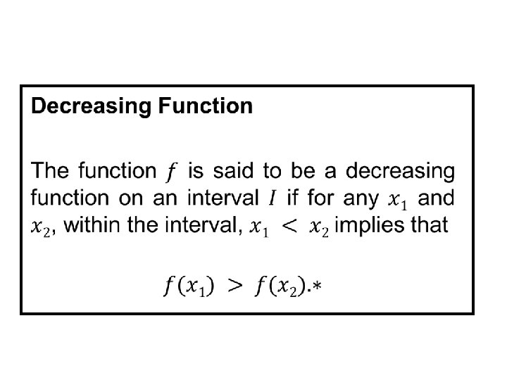
• As with increasing functions, decreasing functions can be identified by tangent slope conditions. • If the first derivative of f is negative throughout an interval, then the slope is negative and f is a decreasing function on the interval. • Which means that, at any point within the interval a slight increase in the value of x will be accompanied by a decrease in the value of f(x).

Note If a function is increasing (decreasing) on an interval, the function is increasing (decreasing) at every point within the interval.

The Second Derivative • If f”(x) is negative on an interval I of f, the first derivative is decreasing on I. • Graphically, the slope is decreasing in value, on the interval. • If f”(x) is positive on an interval I of f, the first derivative is increasing on I. • Graphically, the slope is increasing in value, on the interval.

Concavity and Inflection Points Concavity: The graph of a function f is concave up (down) on an interval if f’ increases (decreases) on the entire interval. Inflection Point: A point at which the concavity changes is called an inflection point.

Graphics of Inflection Points

Relationships Between The Second Derivative And Concavity I- If f”(x) < 0 on an interval a ≤ x ≤ b, the graph of f is concave down over that interval. For any point x = c within the interval, f is said to be concave down at [c, f(c)]. II- If f”(x) > 0 on any interval a ≤ x ≤ b, the graph of f is concave up over that interval. For any point x = c within the interval, f is said to be concave up at [c, f(c)].

III- If f”(x) = 0 at any point x = c in the domain of f, no conclusion can be drawn about the concavity at [c, f(c)]

Example •

Locating Inflection Points I- Find all points a where f”(a) = 0. II- If f”(x) change sign when passing through x = a, there is an inflection point at x = a.

Review We started chapter 16. Derivatives: Additional Interpretations • Increasing functions • Decreasing functions • Concavity • Inflection points

Next Lecture • Critical points: Maxima and Minima • The first derivative test • The second derivative test