ARO 309 Astronautics and Spacecraft Design Winter 2014

ARO 309 - Astronautics and Spacecraft Design Winter 2014 Try Lam Cal. Poly Pomona Aerospace Engineering

Lecture 03: Numerical Integrations Chapter TBD

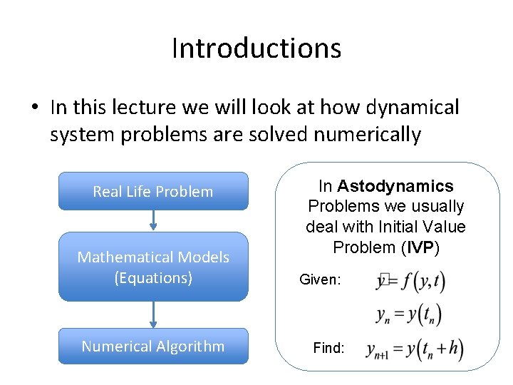
Introductions • In this lecture we will look at how dynamical system problems are solved numerically Real Life Problem In Astodynamics Problems we usually deal with Initial Value Problem (IVP) Mathematical Models (Equations) Given: Numerical Algorithm Find:

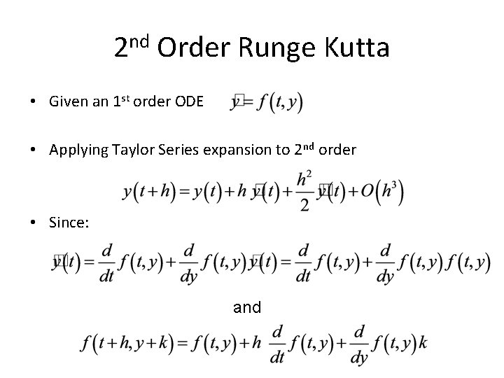
2 nd Order Runge Kutta • Given an 1 st order ODE • Applying Taylor Series expansion to 2 nd order • Since: and

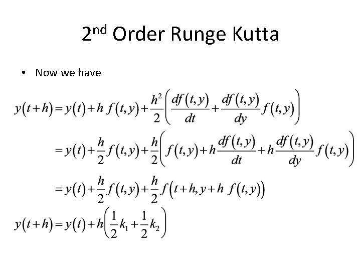
2 nd Order Runge Kutta • Now we have

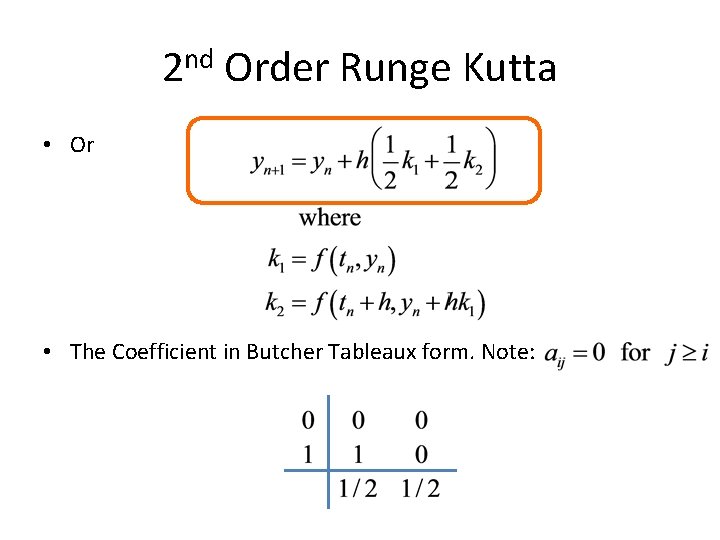
2 nd Order Runge Kutta • Or • The Coefficient in Butcher Tableaux form. Note:

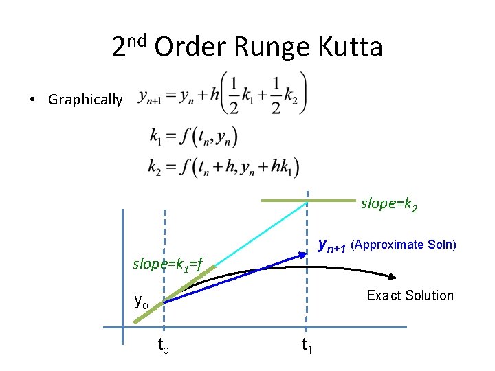
2 nd Order Runge Kutta • Graphically slope=k 2 yn+1 (Approximate Soln) slope=k 1=f Exact Solution yo to t 1

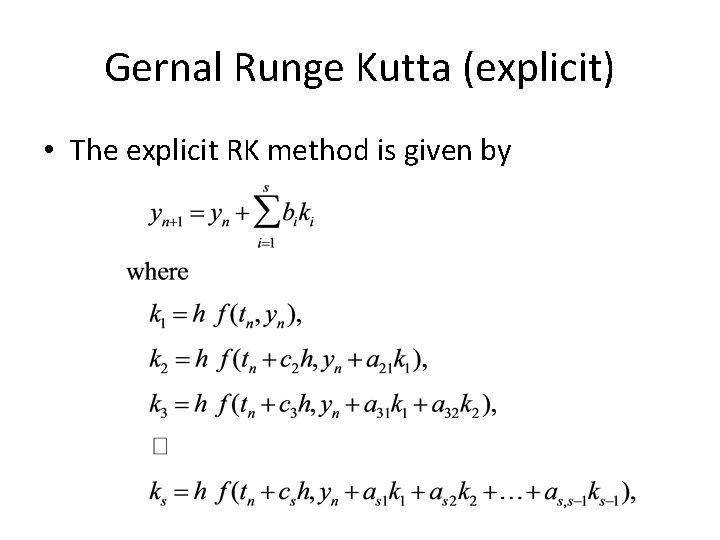
Gernal Runge Kutta (explicit) • The explicit RK method is given by

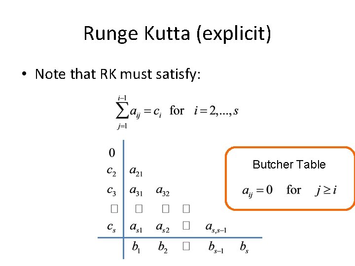
Runge Kutta (explicit) • Note that RK must satisfy: Butcher Table

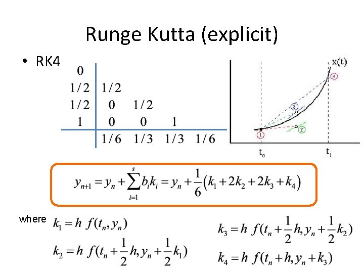
Runge Kutta (explicit) • RK 4 where

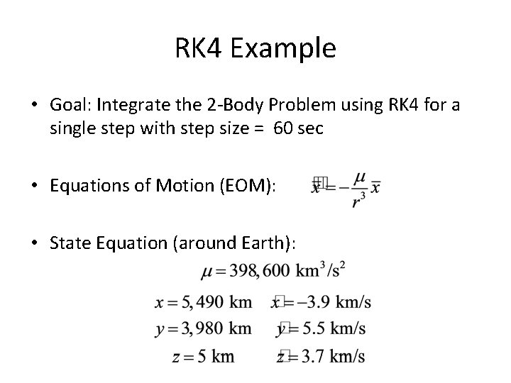
RK 4 Example • Goal: Integrate the 2 -Body Problem using RK 4 for a single step with step size = 60 sec • Equations of Motion (EOM): • State Equation (around Earth):

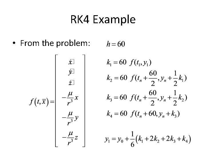
RK 4 Example • From the problem:

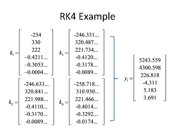
RK 4 Example

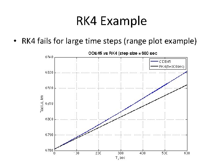
RK 4 Example • RK 4 fails for large time steps (range plot example)

Lecture 04: Two-Body Dynamics: Orbit Position as a Function of Time Chapter 3

Introductions • Chapter 2 (Lection 1 and 2) relates position as a function of θ (true anomaly) but not time • Time was only introduced when referring to orbit period • Here we attempt to find the relations between position of the S/C and time Kepler’s Equation

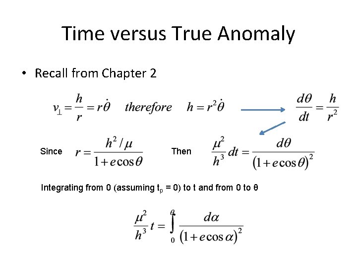
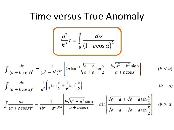
Time versus True Anomaly • Recall from Chapter 2 Since Then Integrating from 0 (assuming tp = 0) to t and from 0 to θ

Time versus True Anomaly

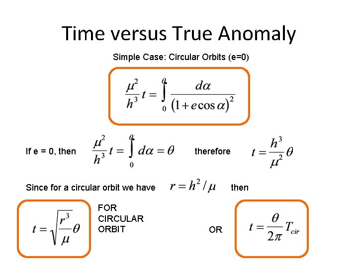
Time versus True Anomaly Simple Case: Circular Orbits (e=0) If e = 0, then therefore Since for a circular orbit we have FOR CIRCULAR ORBIT then OR

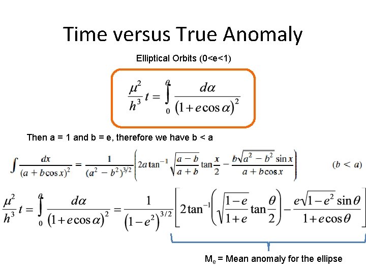
Time versus True Anomaly Elliptical Orbits (0<e<1) Then a = 1 and b = e, therefore we have b < a Me = Mean anomaly for the ellipse

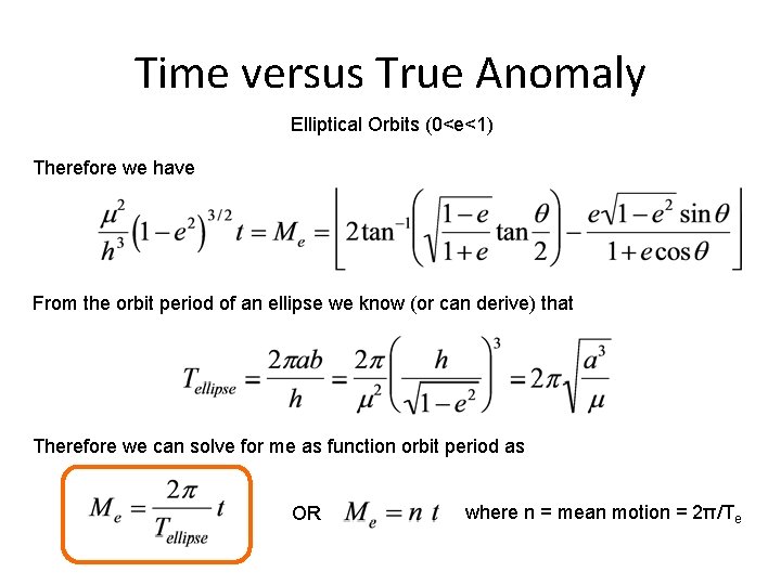
Time versus True Anomaly Elliptical Orbits (0<e<1) Therefore we have From the orbit period of an ellipse we know (or can derive) that Therefore we can solve for me as function orbit period as OR where n = mean motion = 2π/Te

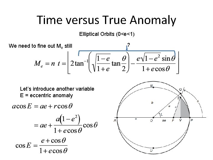
Time versus True Anomaly Elliptical Orbits (0<e<1) We need to fine out Me still Let’s introduce another variable E = eccentric anomaly ?

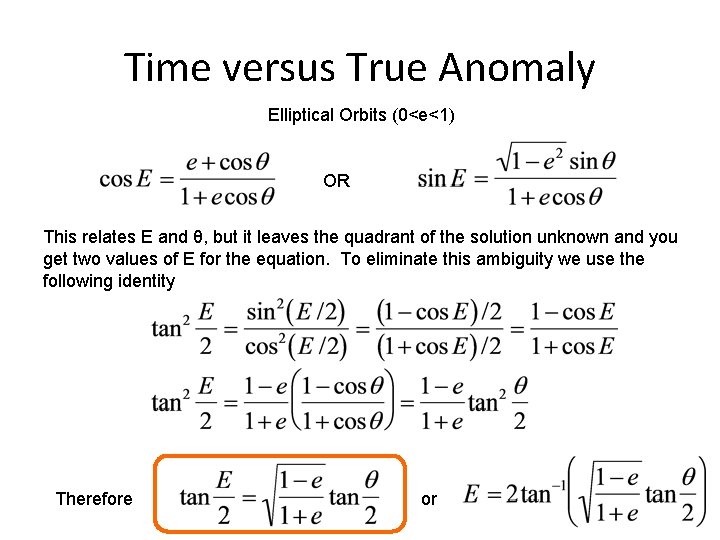
Time versus True Anomaly Elliptical Orbits (0<e<1) OR This relates E and θ, but it leaves the quadrant of the solution unknown and you get two values of E for the equation. To eliminate this ambiguity we use the following identity Therefore or

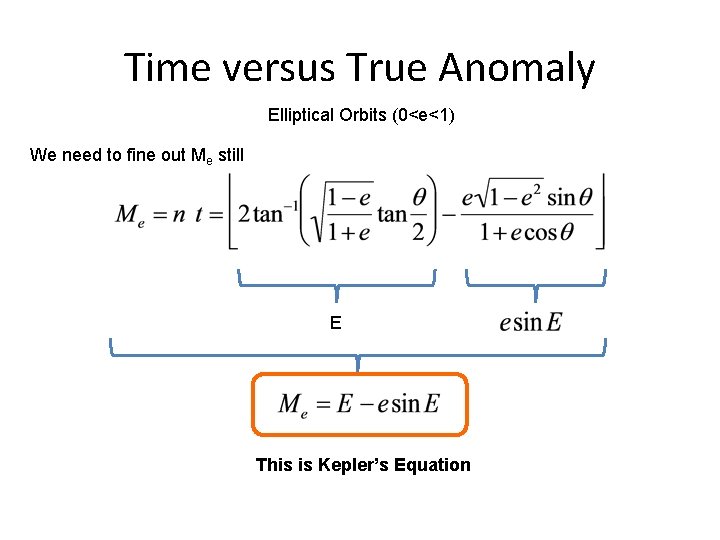
Time versus True Anomaly Elliptical Orbits (0<e<1) We need to fine out Me still E This is Kepler’s Equation

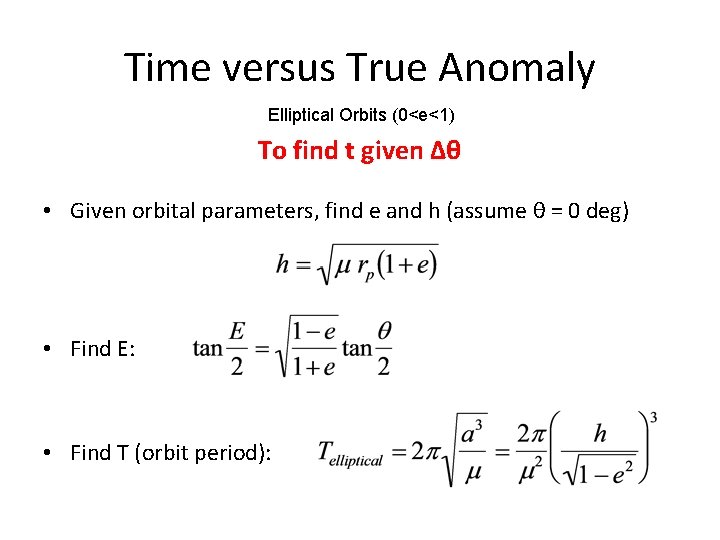
Time versus True Anomaly Elliptical Orbits (0<e<1) To find t given Δθ • Given orbital parameters, find e and h (assume θ = 0 deg) • Find E: • Find T (orbit period):

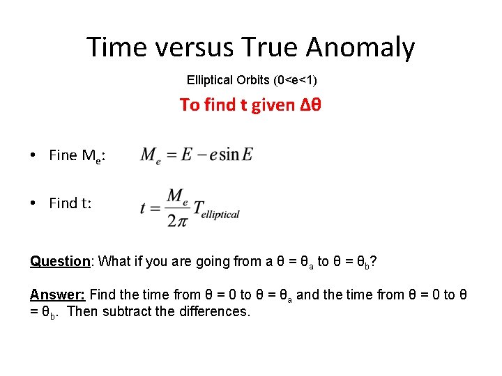
Time versus True Anomaly Elliptical Orbits (0<e<1) To find t given Δθ • Fine Me: • Find t: Question: What if you are going from a θ = θa to θ = θb? Answer: Find the time from θ = 0 to θ = θa and the time from θ = 0 to θ = θb. Then subtract the differences.

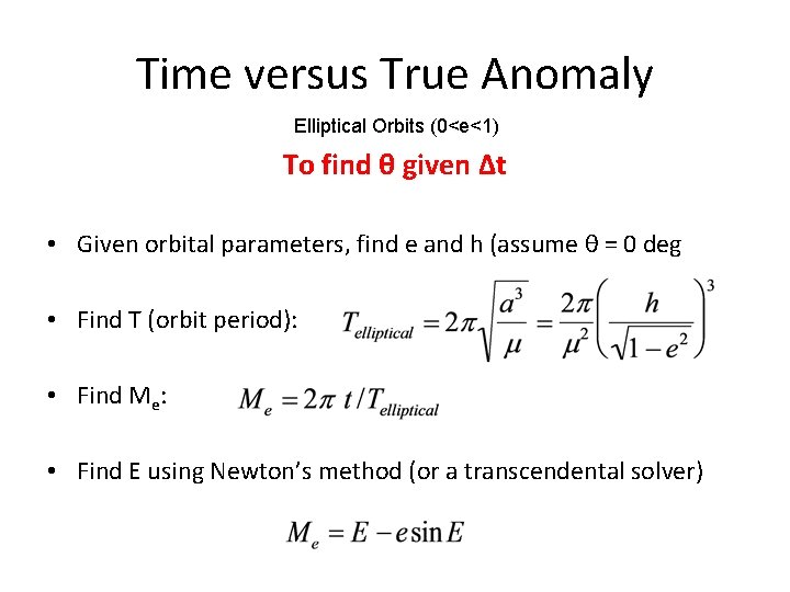
Time versus True Anomaly Elliptical Orbits (0<e<1) To find θ given Δt • Given orbital parameters, find e and h (assume θ = 0 deg • Find T (orbit period): • Find Me: • Find E using Newton’s method (or a transcendental solver)

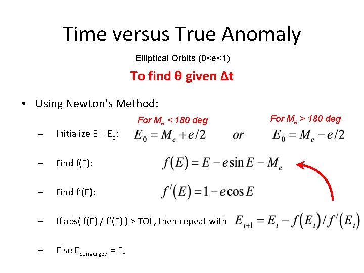
Time versus True Anomaly Elliptical Orbits (0<e<1) To find θ given Δt • Using Newton’s Method: For Me < 180 deg – Initialize E = Eo: – Find f(E): – Find f’(E): – If abs( f(E) / f’(E) ) > TOL, then repeat with – Else Econverged = En For Me > 180 deg

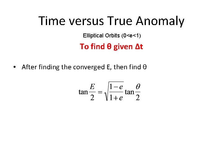
Time versus True Anomaly Elliptical Orbits (0<e<1) To find θ given Δt • After finding the converged E, then find θ

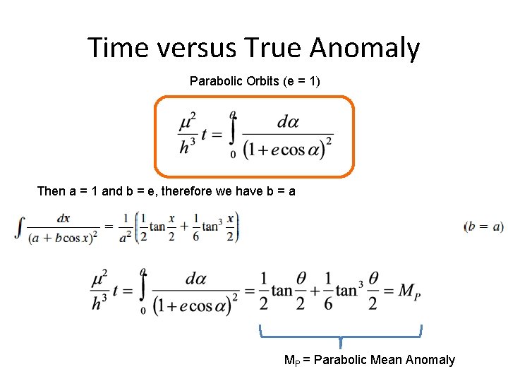
Time versus True Anomaly Parabolic Orbits (e = 1) Then a = 1 and b = e, therefore we have b = a MP = Parabolic Mean Anomaly

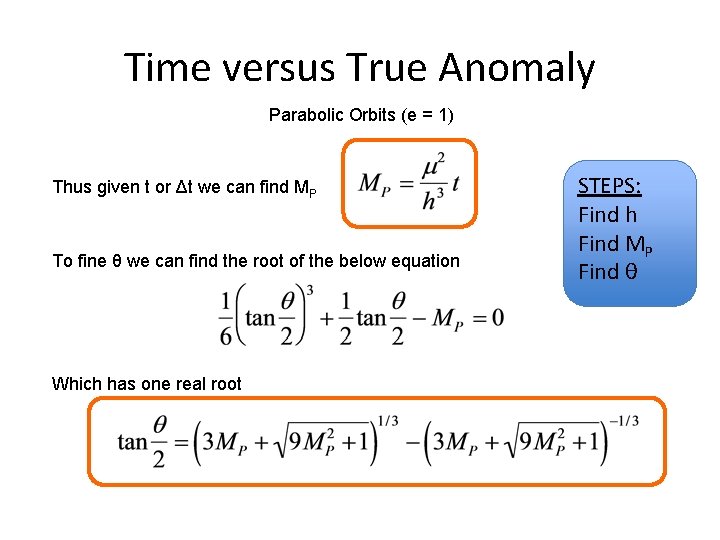
Time versus True Anomaly Parabolic Orbits (e = 1) Thus given t or Δt we can find MP To fine θ we can find the root of the below equation Which has one real root STEPS: Find h Find MP Find θ

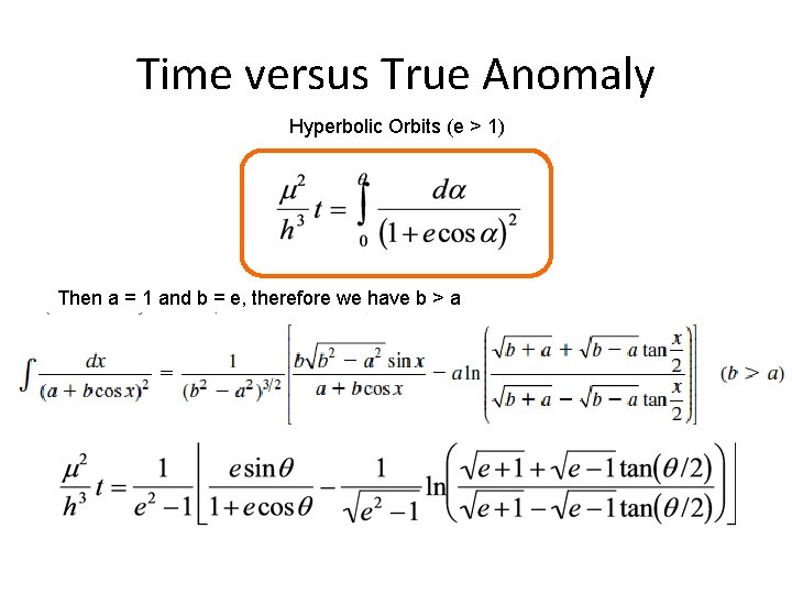
Time versus True Anomaly Hyperbolic Orbits (e > 1) Then a = 1 and b = e, therefore we have b > a

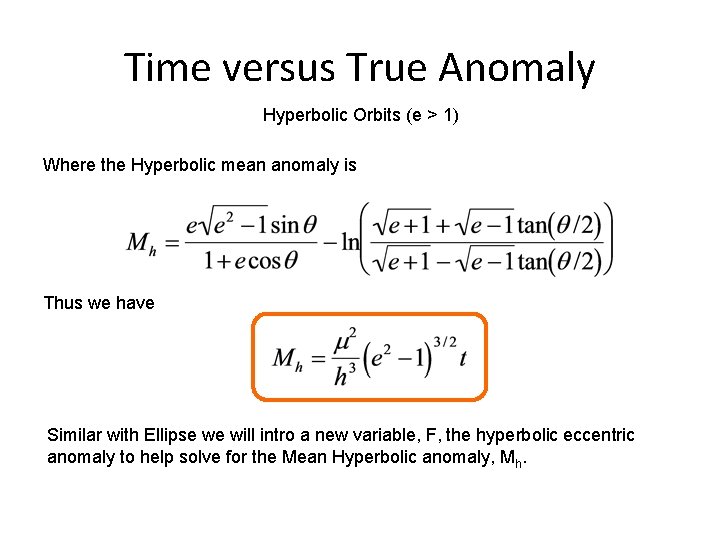
Time versus True Anomaly Hyperbolic Orbits (e > 1) Where the Hyperbolic mean anomaly is Thus we have Similar with Ellipse we will intro a new variable, F, the hyperbolic eccentric anomaly to help solve for the Mean Hyperbolic anomaly, Mh.

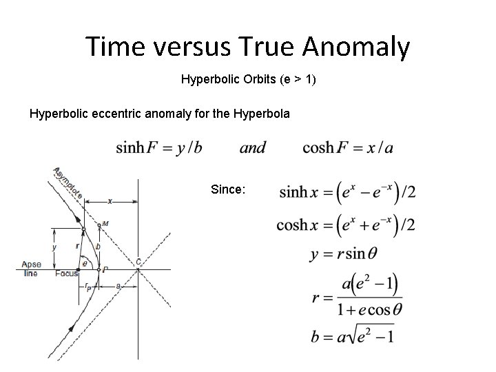
Time versus True Anomaly Hyperbolic Orbits (e > 1) Hyperbolic eccentric anomaly for the Hyperbola Since:

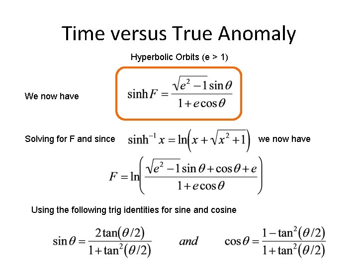
Time versus True Anomaly Hyperbolic Orbits (e > 1) We now have Solving for F and since Using the following trig identities for sine and cosine we now have

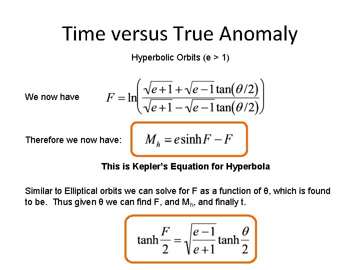
Time versus True Anomaly Hyperbolic Orbits (e > 1) We now have Therefore we now have: This is Kepler’s Equation for Hyperbola Similar to Elliptical orbits we can solve for F as a function of θ, which is found to be. Thus given θ we can find F, and Mh, and finally t.

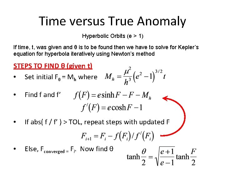
Time versus True Anomaly Hyperbolic Orbits (e > 1) If time, t, was given and θ is to be found then we have to solve for Kepler’s equation for hyperbola iteratively using Newton’s method STEPS TO FIND θ (given t) • Set initial F 0 = Mh where • Find f and f’ • If abs( f / f’ ) > TOL, repeat steps with updated F • Else, Fconverged = Fi. Now find θ

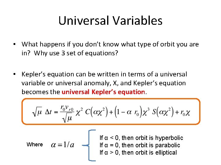
Universal Variables • What happens if you don’t know what type of orbit you are in? Why use 3 set of equations? • Kepler’s equation can be written in terms of a universal variable or universal anomaly, Χ, and Kepler’s equation becomes the universal Kepler’s equation. Where If α < 0, then orbit is hyperbolic If α = 0, then orbit is parabolic If α > 0, then orbit is elliptical

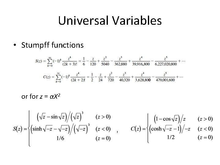
Universal Variables • Stumpff functions or for z = αΧ 2 ,

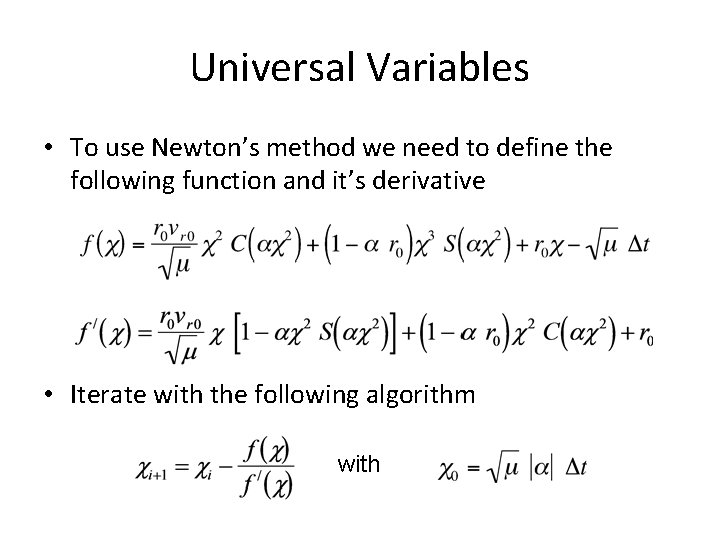
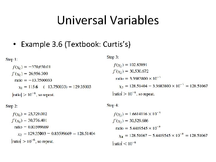
Universal Variables • To use Newton’s method we need to define the following function and it’s derivative • Iterate with the following algorithm with

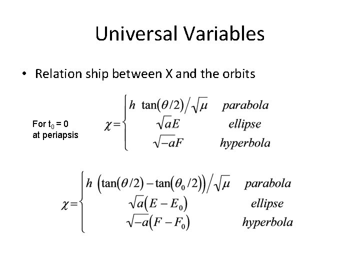
Universal Variables • Relation ship between X and the orbits For t 0 = 0 at periapsis

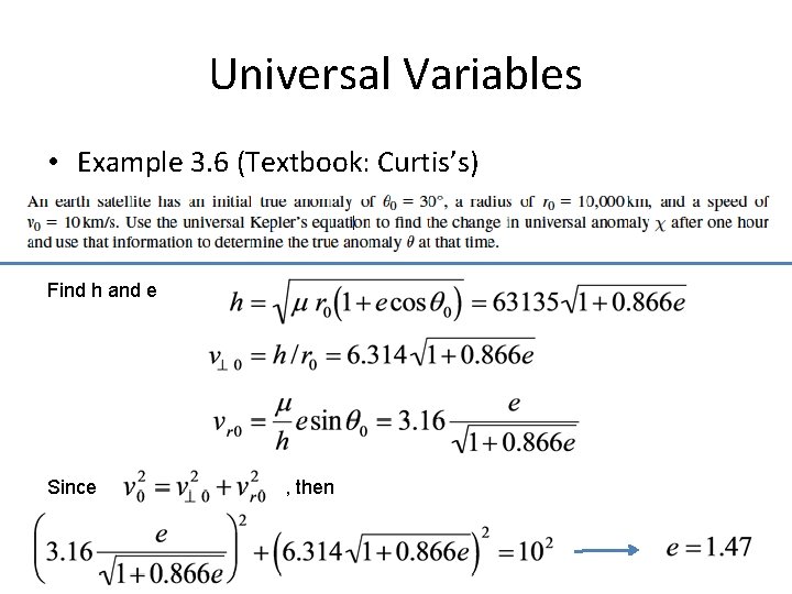
Universal Variables • Example 3. 6 (Textbook: Curtis’s) Find h and e Since , then

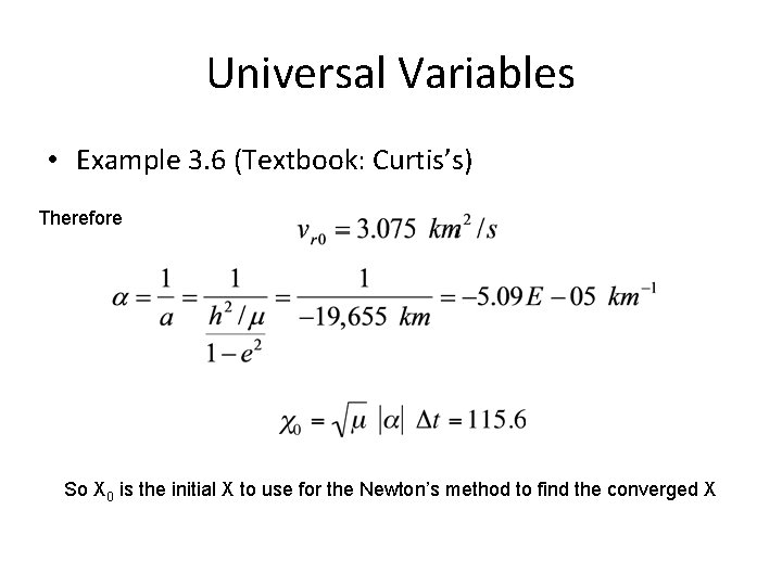
Universal Variables • Example 3. 6 (Textbook: Curtis’s) Therefore So X 0 is the initial X to use for the Newton’s method to find the converged X

Universal Variables • Example 3. 6 (Textbook: Curtis’s)

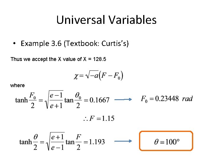
Universal Variables • Example 3. 6 (Textbook: Curtis’s) Thus we accept the X value of X = 128. 5 where

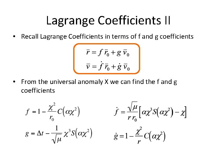
Lagrange Coefficients II • Recall Lagrange Coefficients in terms of f and g coefficients • From the universal anomaly X we can find the f and g coefficients

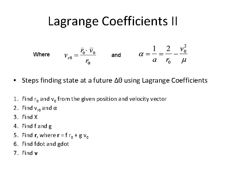
Lagrange Coefficients II Where and • Steps finding state at a future Δθ using Lagrange Coefficients 1. 2. 3. 4. 5. 6. 7. Find r 0 and v 0 from the given position and velocity vector Find vr 0 and α Find X Find f and g Find r, where r = f r 0 + g v 0 Find fdot and gdot Find v