Angular Correlations in Gamma Deexcitation Jason Detwiler Micah

Angular Correlations in Gamma De-excitation Jason Detwiler, Micah Buuck, Ian Guinn, Aobo Li University of Washington March 3, 2015

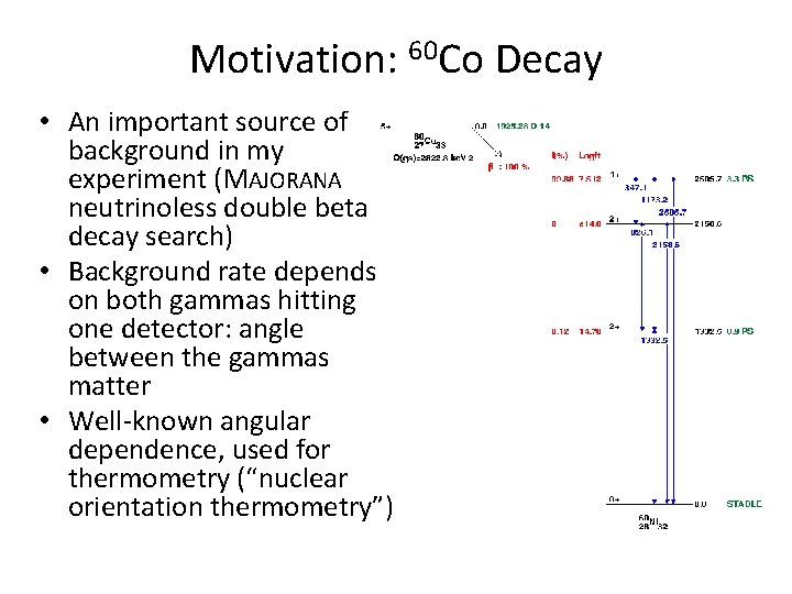
Motivation: 60 Co Decay • An important source of background in my experiment (MAJORANA neutrinoless double beta decay search) • Background rate depends on both gammas hitting one detector: angle between the gammas matter • Well-known angular dependence, used for thermometry (“nuclear orientation thermometry”)

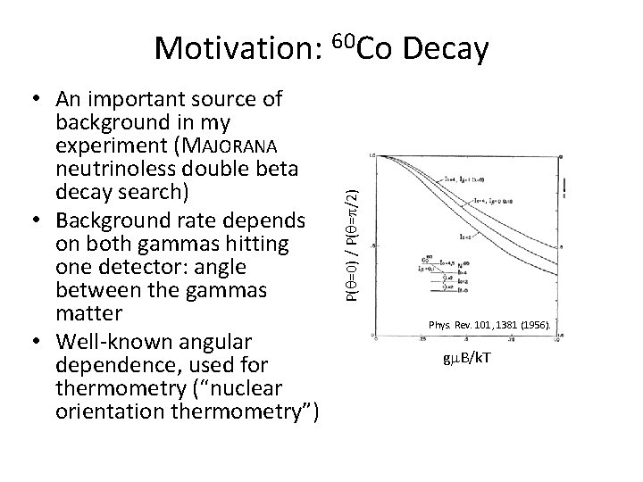
• An important source of background in my experiment (MAJORANA neutrinoless double beta decay search) • Background rate depends on both gammas hitting one detector: angle between the gammas matter • Well-known angular dependence, used for thermometry (“nuclear orientation thermometry”) P(q=0) / P(q=p/2) Motivation: 60 Co Decay Phys. Rev. 101, 1381 (1956). gm. B/k. T

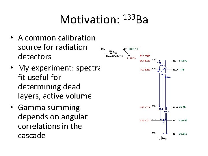
Motivation: 133 Ba • A common calibration source for radiation detectors • My experiment: spectral fit useful for determining dead layers, active volume • Gamma summing depends on angular correlations in the cascade

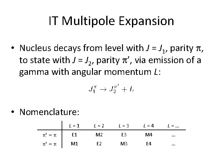
IT Multipole Expansion • Nucleus decays from level with J = J 1, parity p, to state with J = J 2, parity p’, via emission of a gamma with angular momentum L: • Nomenclature: L=1 L=2 L=3 L=4 L=… p’ = p E 1 M 2 E 3 M 4 … p’ = p M 1 E 2 M 3 E 4 …

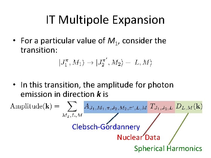
IT Multipole Expansion • For a particular value of M 1, consider the transition: • In this transition, the amplitude for photon emission in direction k is Clebsch-Gordannery • To include all M 1, sum over the density matrix for Nuclear the nuclear polarization states and Data square to get the probability for emission in direction Sphericalk. Harmonics

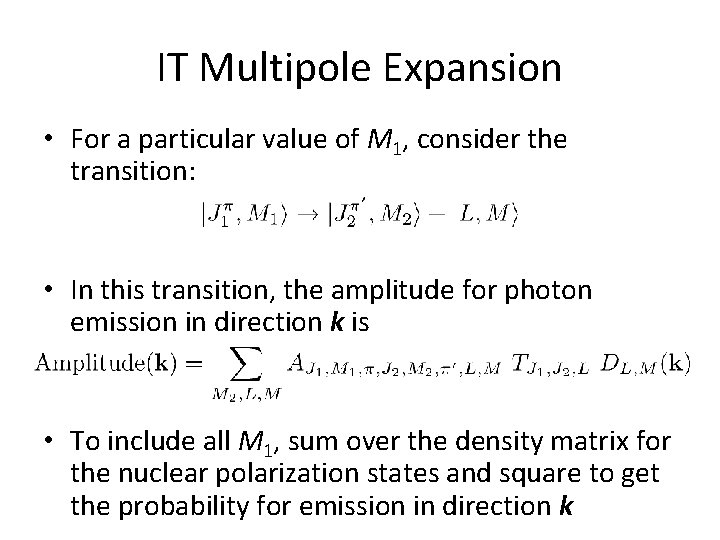
IT Multipole Expansion • For a particular value of M 1, consider the transition: • In this transition, the amplitude for photon emission in direction k is • To include all M 1, sum over the density matrix for the nuclear polarization states and square to get the probability for emission in direction k

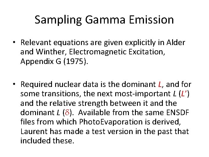
Sampling Gamma Emission • Relevant equations are given explicitly in Alder and Winther, Electromagnetic Excitation, Appendix G (1975). • Required nuclear data is the dominant L, and for some transitions, the next most-important L (L’) and the relative strength between it and the dominant L (d). Available from the same ENSDF files from which Photo. Evaporation is derived, Laurent has made a test version in the past that included these.

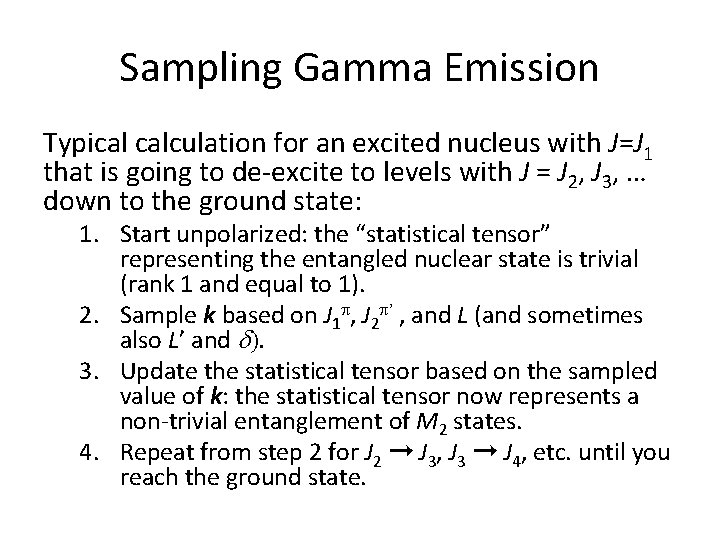
Sampling Gamma Emission Typical calculation for an excited nucleus with J=J 1 that is going to de-excite to levels with J = J 2, J 3, … down to the ground state: 1. Start unpolarized: the “statistical tensor” representing the entangled nuclear state is trivial (rank 1 and equal to 1). 2. Sample k based on J 1 p, J 2 p’ , and L (and sometimes also L’ and d). 3. Update the statistical tensor based on the sampled value of k: the statistical tensor now represents a non-trivial entanglement of M 2 states. 4. Repeat from step 2 for J 2 ➞ J 3, J 3 ➞ J 4, etc. until you reach the ground state.

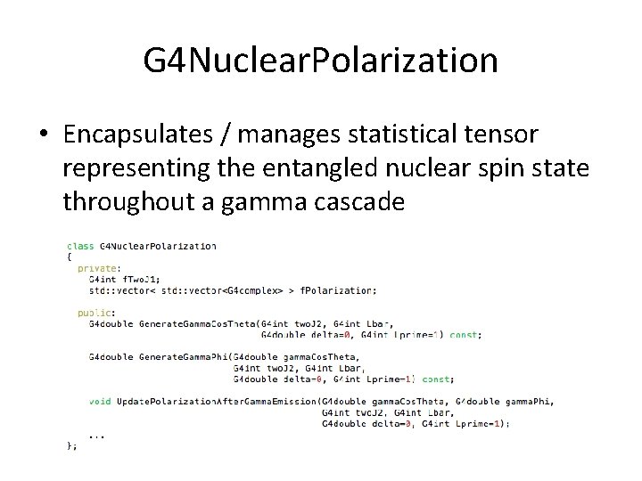
G 4 Nuclear. Polarization • Encapsulates / manages statistical tensor representing the entangled nuclear spin state throughout a gamma cascade

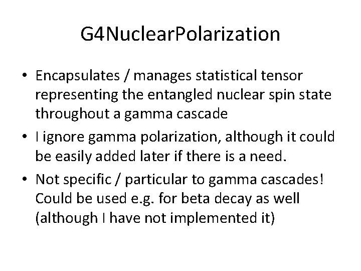
G 4 Nuclear. Polarization • Encapsulates / manages statistical tensor representing the entangled nuclear spin state throughout a gamma cascade • I ignore gamma polarization, although it could be easily added later if there is a need. • Not specific / particular to gamma cascades! Could be used e. g. for beta decay as well (although I have not implemented it)

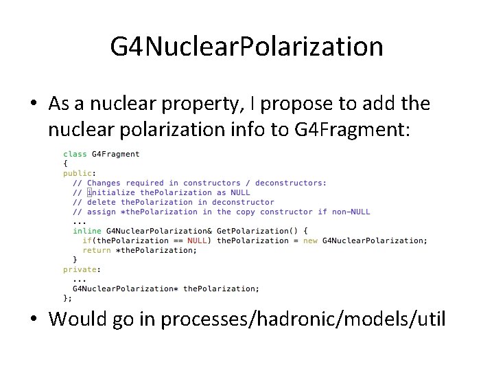
G 4 Nuclear. Polarization • As a nuclear property, I propose to add the nuclear polarization info to G 4 Fragment: • Would go in processes/hadronic/models/util

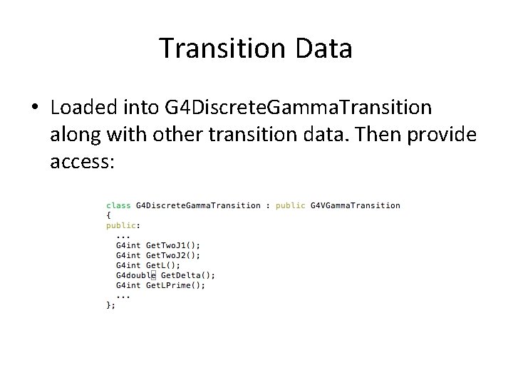
Transition Data • Loaded into G 4 Discrete. Gamma. Transition along with other transition data. Then provide access:

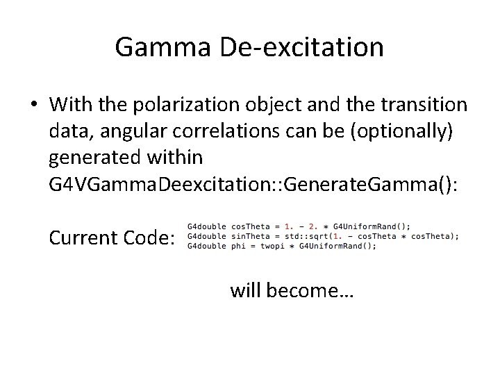
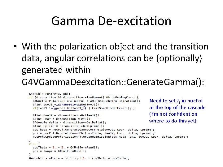
Gamma De-excitation • With the polarization object and the transition data, angular correlations can be (optionally) generated within G 4 VGamma. Deexcitation: : Generate. Gamma(): Current Code: will become…

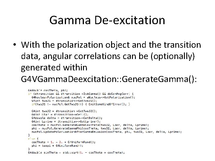
Gamma De-excitation • With the polarization object and the transition data, angular correlations can be (optionally) generated within G 4 VGamma. Deexcitation: : Generate. Gamma():

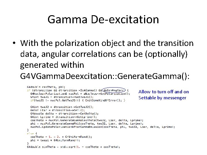
Gamma De-excitation • With the polarization object and the transition data, angular correlations can be (optionally) generated within G 4 VGamma. Deexcitation: : Generate. Gamma(): Allow to turn off and on Settable by messenger

Gamma De-excitation • With the polarization object and the transition data, angular correlations can be (optionally) generated within G 4 VGamma. Deexcitation: : Generate. Gamma(): Need to set J 1 in nuc. Pol at the top of the cascade (I’m not confident on where to do this yet)

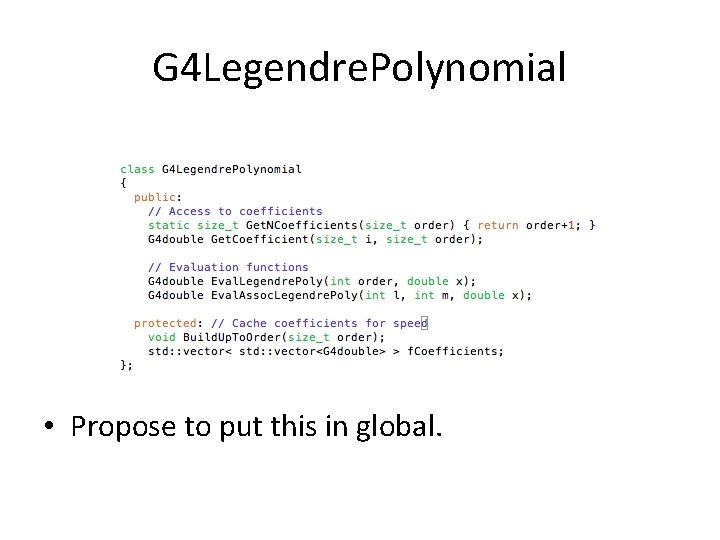
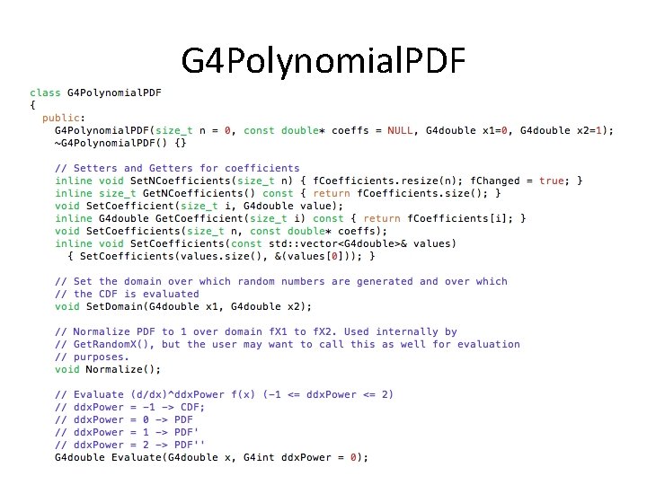
Additional Required Tools • Angular momentum coupling: need to compute Wigner 3 J, 6 J and 9 J symbols – G 4 Clebsch has 3 J but not the others – gsl has these but G 4 doesn’t useful things like gsl • Angular distributions: need to compute associated Legendre polynomials – neutron/particle_hp have Legendre polynomials but not associated Legendre polynomials – CLHEP seems to have at least most of what is needed but the paired-down version in G 4 does not include CLHEP’s Legendre polynomial code – gsl also has these… • Random number generation: need to sample from simple polynomial functions – Surprised not to find generic code for generating random numbers from a simple polynomial, not in G 4 or in CLHEP. Maybe I didn’t look hard enough.

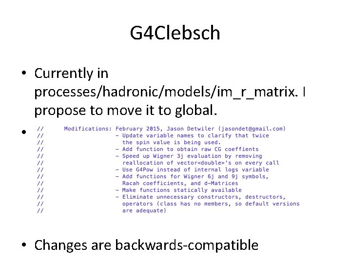
G 4 Clebsch • Currently in processes/hadronic/models/im_r_matrix. I propose to move it to global. • My change log: • Changes are backwards-compatible

G 4 Clebsch Testing • Generate 3 lists of parameters and solutions for each Wigner symbol (3 J, 6 J, 9 J) – Exhaustively scan through all angular momenta up to J = 5 that satisfy selection rules – Generate random sets of parameters up to J = 10 that do not need to satisfy selection rules • Comparison to gsl: – Found bug in gsl: https: //savannah. gnu. org/bugs/? 29606 • Comparison to Mathematica: – For 9 -j symbol, used angular. m notebook by Andrei Derevianko (University of Nevada, Reno) – Agreed to within a few parts in 10 -12 for all values tests, and to within machine precision for all cases of physical relevance (lower J)

G 4 Legendre. Polynomial • Propose to put this in global.

G 4 Legendre. Polynomial Testing 1. Generate Associated Legendre Polynomials with Mathematica through l=30 – Coefficients – Evaluations at random x-values 2. Compare to results from G 4 Legendre. Polynomial – Coefficients and evaluations agree to within machine precision

G 4 Polynomial. PDF

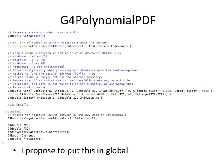
G 4 Polynomial. PDF • I propose to put this in global

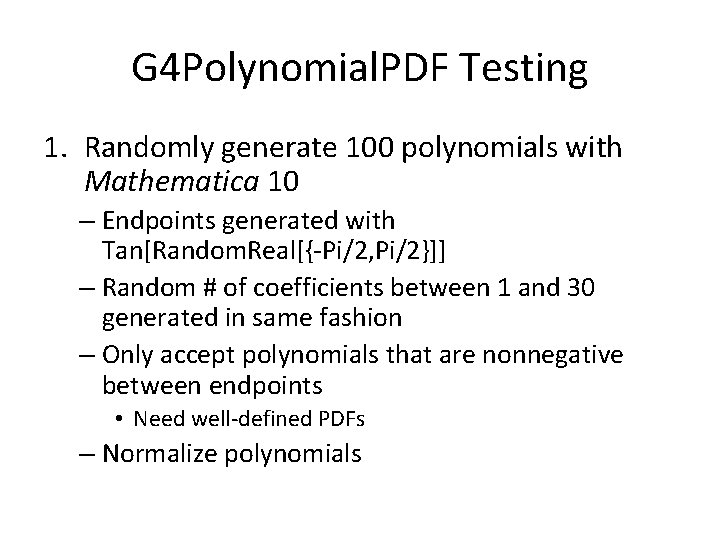
G 4 Polynomial. PDF Testing 1. Randomly generate 100 polynomials with Mathematica 10 – Endpoints generated with Tan[Random. Real[{-Pi/2, Pi/2}]] – Random # of coefficients between 1 and 30 generated in same fashion – Only accept polynomials that are nonnegative between endpoints • Need well-defined PDFs – Normalize polynomials

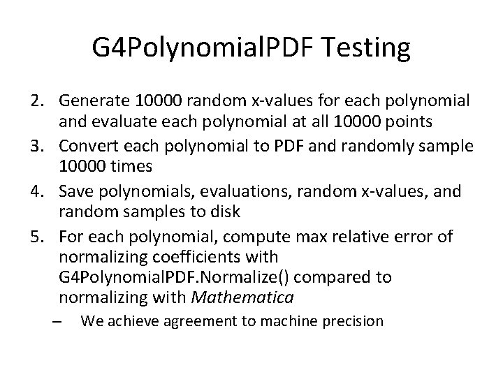
G 4 Polynomial. PDF Testing 2. Generate 10000 random x-values for each polynomial and evaluate each polynomial at all 10000 points 3. Convert each polynomial to PDF and randomly sample 10000 times 4. Save polynomials, evaluations, random x-values, and random samples to disk 5. For each polynomial, compute max relative error of normalizing coefficients with G 4 Polynomial. PDF. Normalize() compared to normalizing with Mathematica – We achieve agreement to machine precision

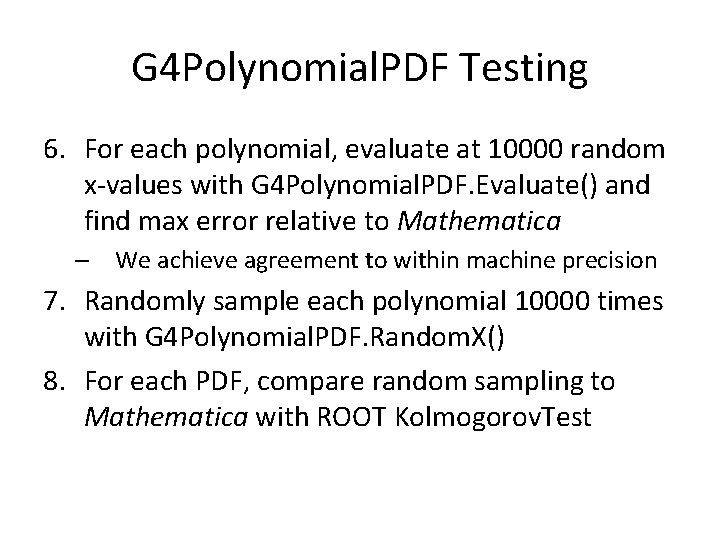
G 4 Polynomial. PDF Testing 6. For each polynomial, evaluate at 10000 random x-values with G 4 Polynomial. PDF. Evaluate() and find max error relative to Mathematica – We achieve agreement to within machine precision 7. Randomly sample each polynomial 10000 times with G 4 Polynomial. PDF. Random. X() 8. For each PDF, compare random sampling to Mathematica with ROOT Kolmogorov. Test

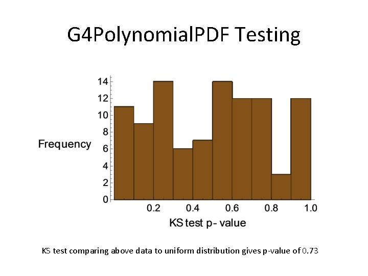
G 4 Polynomial. PDF Testing KS test comparing above data to uniform distribution gives p-value of 0. 73

G 4 Nuclear. Polarization Testing • Rough test: checked that it generates correct polynomials for simple cases • Deep low-level test: check that it generates correct PDFs for multi-level cascades with high J 1 / J 2 / L (highly non-trivial entangled polarization state) • High-level test: generate 60 Co decay and “measure” the angular distribution produced by G 4

G 4 Nuclear. Polarization Low-Level Testing • Generate spherical distributions for three successive gammas emitted by nucleus – First gamma establishes polar axis – Second gamma establishes azimuthal axis – Distribution of angle between first and third gamma can be calculated by integrating out second gamma

G 4 Nuclear. Polarization Low-Level Testing 1. Code analytical expression for polarization tensor in Mathematica – From Alder and Winther 2. Compare theoretical prediction to Falkoff, Phys Rev 82, 98 (1951). – Good agreement, so Mathematica expression seems coded correctly • Integrated squared error of 1. 6 E-7 (over 4π solid angle)

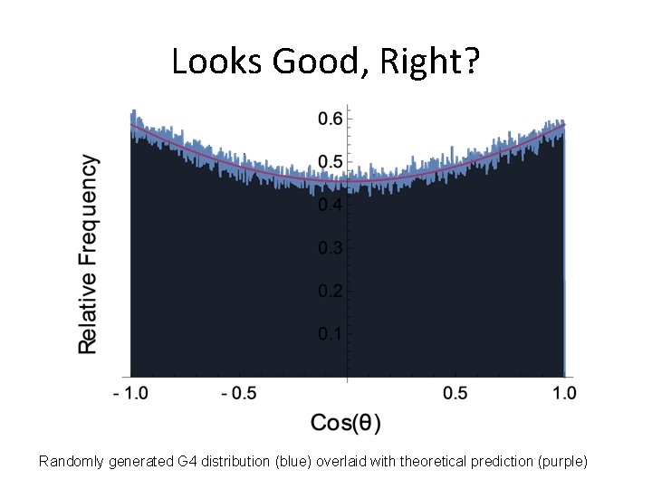
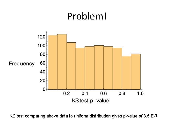
G 4 Nuclear. Polarization Low-Level Testing 3. Compute polarization tensor in Mathematica for gamma triple cascade – Calculate distribution of angle between 1 st and 3 rd gamma. – Generate 1000 angle distributions with 1000 samples in each distribution 4. Use G 4 Nuclear. Polarization to generate 1000 gammas from this transition 1000 times – Compute 1000 KS statistics between G 4 and Mathematica generated distributions

Looks Good, Right? Randomly generated G 4 distribution (blue) overlaid with theoretical prediction (purple)

Problem! KS test comparing above data to uniform distribution gives p-value of 3. 5 E-7

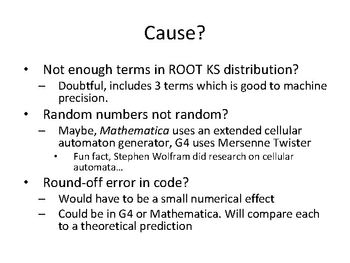
Cause? • Not enough terms in ROOT KS distribution? – Doubtful, includes 3 terms which is good to machine precision. • Random numbers not random? – Maybe, Mathematica uses an extended cellular automaton generator, G 4 uses Mersenne Twister • Fun fact, Stephen Wolfram did research on cellular automata… • Round-off error in code? – Would have to be a small numerical effect – Could be in G 4 or Mathematica. Will compare each to a theoretical prediction

G 4 Nuclear. Polarization High-Level Testing • Use G 4 RDM to generate nuclear decay at the center of a spherical vacuum. • Tag gamma positions as they exit the sphere • Histogram angular correlations and compare to theoretical expectations • Setup is up-and-running, verified that G 4 indeed generates isotropic gammas • Need to finish implementation and obtain custom Photo. Evaporation data files to proceed

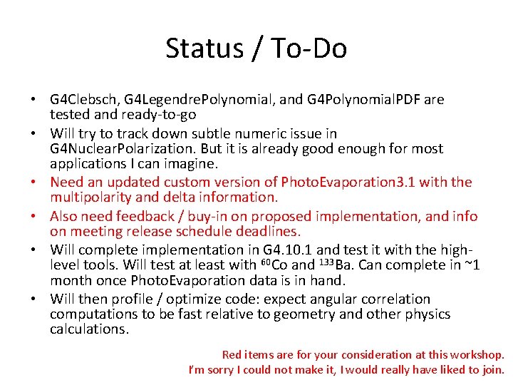
Status / To-Do • G 4 Clebsch, G 4 Legendre. Polynomial, and G 4 Polynomial. PDF are tested and ready-to-go • Will try to track down subtle numeric issue in G 4 Nuclear. Polarization. But it is already good enough for most applications I can imagine. • Need an updated custom version of Photo. Evaporation 3. 1 with the multipolarity and delta information. • Also need feedback / buy-in on proposed implementation, and info on meeting release schedule deadlines. • Will complete implementation in G 4. 10. 1 and test it with the highlevel tools. Will test at least with 60 Co and 133 Ba. Can complete in ~1 month once Photo. Evaporation data is in hand. • Will then profile / optimize code: expect angular correlation computations to be fast relative to geometry and other physics calculations. Red items are for your consideration at this workshop. I’m sorry I could not make it, I would really have liked to join.