Algorithmic and Statistical Perspectives on LargeScale Data Analysis

Algorithmic and Statistical Perspectives on Large-Scale Data Analysis Michael W. Mahoney Stanford University Feb 2010 ( For more info, see: http: // cs. stanford. edu/people/mmahoney/ or Google on “Michael Mahoney”)

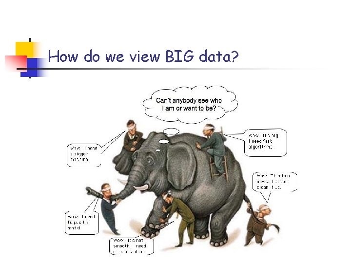
How do we view BIG data?

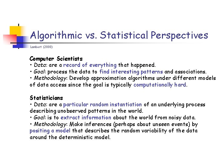
Algorithmic vs. Statistical Perspectives Lambert (2000) Computer Scientists • Data: are a record of everything that happened. • Goal: process the data to find interesting patterns and associations. • Methodology: Develop approximation algorithms under different models of data access since the goal is typically computationally hard. Statisticians • Data: are a particular random instantiation of an underlying process describing unobserved patterns in the world. • Goal: is to extract information about the world from noisy data. • Methodology: Make inferences (perhaps about unseen events) by positing a model that describes the random variability of the data around the deterministic model.

Perspectives are NOT incompatible • Statistical/probabilistic ideas are central to recent work on developing improved randomized algorithms for matrix problems. • Intractable optimization problems on graphs/networks yield to approximation when assumptions are made about network participants. • In boosting (a statistical technique that fits an additive model by minimizing an objective function with a method such as gradient descent), the computation parameter (i. e. , the number of iterations) also serves as a regularization parameter.

Matrices and graphs in data analysis Graphs: • model information network with graph G = (V, E) -- vertices represent “entities” and edges represent “interactions” between pairs of entities Matrices: • model data sets by a matrix -- since an m x n matrix A can encode information about m objects, each of which is described by n features Matrices and graphs represent a nice tradeoff between: • descriptive flexibility • algorithmic tractability But, the issues that arise are very different than in traditional linear algebra or graph theory …

The gap between NLA and TCS … (… was the genesis of MMDS!) Matrix factorizations: • in NLA and scientific computing - used to express a problem s. t. it can be solved more easily. • in TCS and statistical data analysis - used to represent structure that may be present in a matrix obtained from object-feature observations. NLA: • emphasis on optimal conditioning, • backward error analysis issues, • is running time a large or small constant multiplied by n 2 or n 3. TCS: • originally motivated by large data applications • consider space-constrained or pass-efficient models • exploiting over-sampling and randomness as computational resources.

Outline • “Algorithmic” and “statistical” perspectives on data problems • Genetics application DNA SNP analysis --> choose columns from a matrix PMJKPGKD, Genome Research ’ 07; PZBCRMD, PLOS Genetics ’ 07; Mahoney and Drineas, PNAS ’ 09; DMM, SIMAX ‘ 08; BMD, SODA ‘ 09 • Internet application Community finding --> partitioning a graph LLDM (WWW ‘ 08 & TR-Jrnl ‘ 08 & WWW ‘ 10) We will focus on what was going on “under the hood” in these two applications --- use statistical properties implicit in worst-case algorithms to make domain-specific claims!

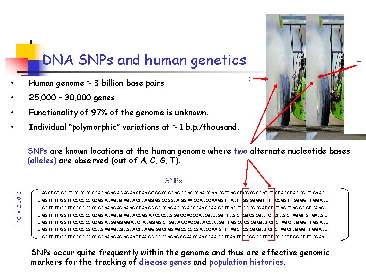
DNA SNPs and human genetics T C • Human genome ≈ 3 billion base pairs • 25, 000 – 30, 000 genes • Functionality of 97% of the genome is unknown. • Individual “polymorphic” variations at ≈ 1 b. p. /thousand. SNPs are known locations at the human genome where two alternate nucleotide bases (alleles) are observed (out of A, C, G, T). individuals SNPs … AG CT GT GG CT CC CC AG AG AG AA CT AA GG GG CC GG AG CG AC CC AA GG TT AG CT CG CG CG AT CT CT AG GG GT GA AG … … GG TT TT GG TT CC CC GG AA AG AG AG AA CT AA GG GG CC GG AA CC AA GG TT AA TT GG GG GG TT TT CC GG TT GG AA … … GG TT TT GG TT CC CC GG AA AG AG AA AG CT AA GG GG CC AG AG CG AC CC AA GG TT AG CT CG CG CG AT CT CT AG GG GT GA AG … … GG TT TT GG TT CC CC GG AA AG AG AG AA CC GG AA CC CC AG GG CC AC CC AA CG AA GG TT AG CT CG CG CG AT CT CT AG GT GT GA AG … … GG TT TT GG TT CC CC GG AA GG GG GG AA CT AA GG GG CT GG AA CC AC CG AA CC AA GG TT GG CC CG CG CG AT CT CT AG GG TT GG AA … … GG TT TT GG TT CC CC CG CC AG AG AG AA CT AA GG GG CT GG AG CC CC CG AA CC AA GT TT AG CT CG CG CG AT CT CT AG GG TT GG AA … … GG TT TT GG TT CC CC GG AA AG AG AG AA TT AA GG GG CC AG AG CG AA CC AA CG AA GG TT AA TT GG GG GG TT TT CC GG TT GG GT TT GG AA … SNPs occur quite frequently within the genome and thus are effective genomic markers for the tracking of disease genes and population histories.

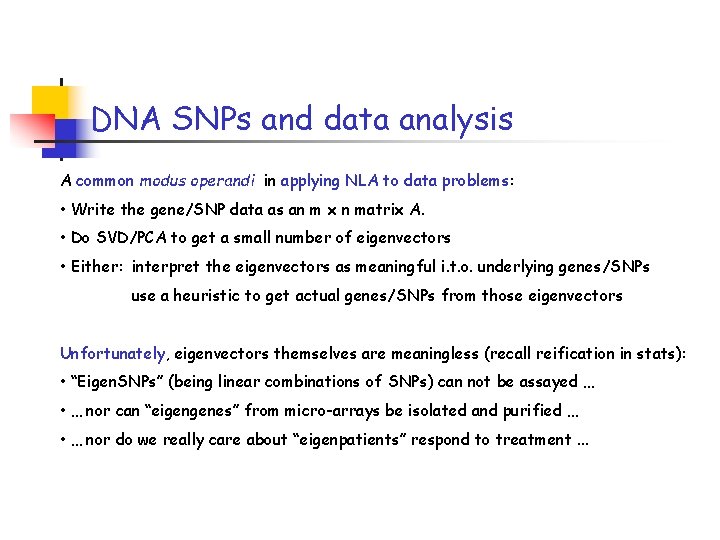
DNA SNPs and data analysis A common modus operandi in applying NLA to data problems: • Write the gene/SNP data as an m x n matrix A. • Do SVD/PCA to get a small number of eigenvectors • Either: interpret the eigenvectors as meaningful i. t. o. underlying genes/SNPs use a heuristic to get actual genes/SNPs from those eigenvectors Unfortunately, eigenvectors themselves are meaningless (recall reification in stats): • “Eigen. SNPs” (being linear combinations of SNPs) can not be assayed … • … nor can “eigengenes” from micro-arrays be isolated and purified … • … nor do we really care about “eigenpatients” respond to treatment. . .

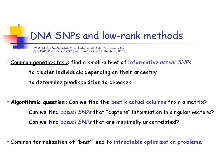
DNA SNPs and low-rank methods PMJKPGKD, Genome Research ’ 07 (data from K. Kidd, Yale University) PZBCRMD, PLOS Genetics ’ 07 (data from E. Ziv and E. Burchard, UCSF) • Common genetics task: find a small subset of informative actual SNPs to cluster individuals depending on their ancestry to determine predisposition to diseases • Algorithmic question: Can we find the best k actual columns from a matrix? Can we find actual SNPs that “capture” information in singular vectors? Can we find actual SNPs that are maximally uncorrelated? • Common formalization of “best” lead to intractable optimization problems.

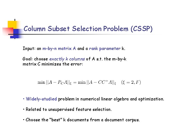
Column Subset Selection Problem (CSSP) Input: an m-by-n matrix A and a rank parameter k. Goal: choose exactly k columns of A s. t. the m-by-k matrix C minimizes the error: • Widely-studied problem in numerical linear algebra and optimization. • Related to unsupervised feature selection. • Choose the “best” k documents from a document corpus.

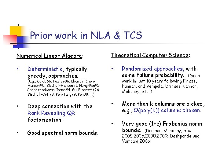
Prior work in NLA & TCS Numerical Linear Algebra: Theoretical Computer Science: • • Deterministic, typically greedy, approaches. work in last 10 years following Frieze, Kannan, and Vempala; Drineas, Kannan, Mahoney, etc. . ) (E. g. , Golub 65, Foster 86, Chan 87, Chan. Hansen 90, Bischof-Hansen 91, Hong-Pan 92, Chandrasekaran-Ipsen 94, Gu-Eisenstat 96, Bischof-Orti 98, Pan-Tang 99, Pan 00, . . . ) • • Deep connection with the Rank Revealing QR factorization. Good spectral norm bounds. Randomized approaches, with some failure probability. (Much • More than k columns are picked, e. g. , O(poly(k)) columns chosen. • Very good (1+ ) Frobenius norm bounds. (Drineas, Mahoney, etc. 2005, 2006, 2008, 2009; Deshpande and Vempala 2006)

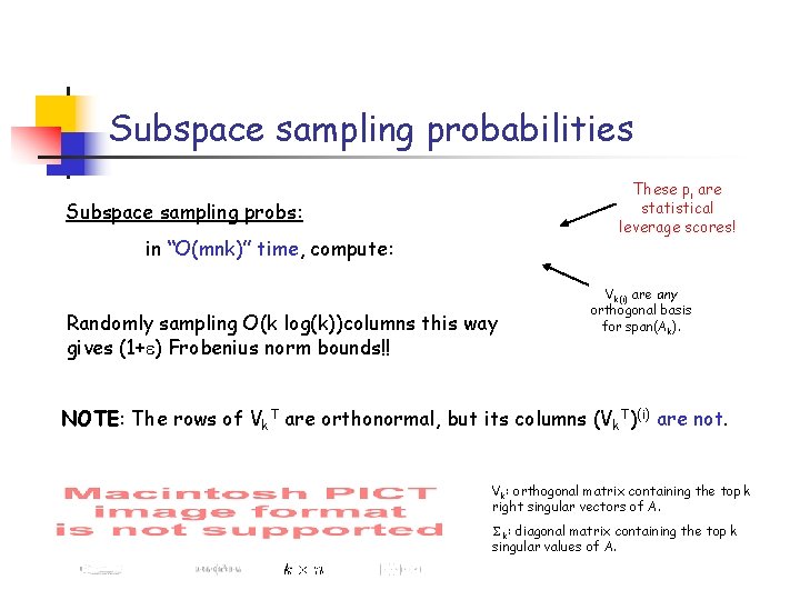
Subspace sampling probabilities These pi are statistical leverage scores! Subspace sampling probs: in “O(mnk)” time, compute: Randomly sampling O(k log(k))columns this way gives (1+ ) Frobenius norm bounds!! Vk(i) are any orthogonal basis for span(Ak). NOTE: The rows of Vk. T are orthonormal, but its columns (Vk. T)(i) are not. Vk: orthogonal matrix containing the top k right singular vectors of A. S k: diagonal matrix containing the top k singular values of A.

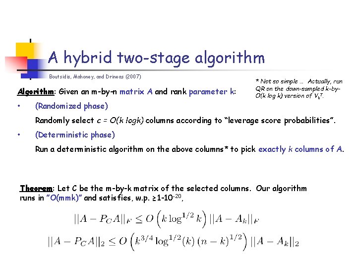
A hybrid two-stage algorithm Boutsidis, Mahoney, and Drineas (2007) Algorithm: Given an m-by-n matrix A and rank parameter k: • (Randomized phase) * Not so simple … Actually, run QR on the down-sampled k-by. O(k log k) version of Vk. T. Randomly select c = O(k logk) columns according to “leverage score probabilities”. • (Deterministic phase) Run a deterministic algorithm on the above columns* to pick exactly k columns of A. Theorem: Let C be the m-by-k matrix of the selected columns. Our algorithm runs in ”O(mmk)” and satisfies, w. p. ≥ 1 -10 -20,

Comparison with previous results Running time is comparable with NLA algorithms. Spectral norm: • Spectral norm bound is k 1/4 log 1/2 k worse than previous work. Frobenius norm: • An efficient algorithmic result at most (k logk)1/2 worse than the previous existential result. NLA usually interested in columns for the bases they span ! Data analysis usually interested in the columns themselves !

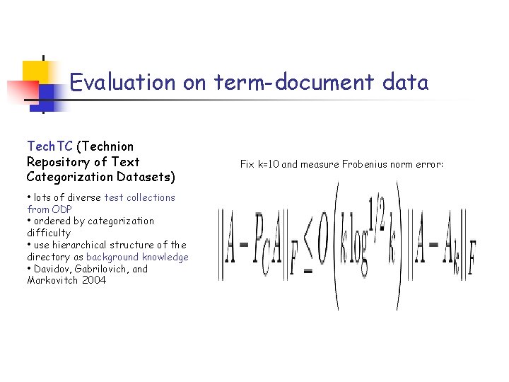
Evaluation on term-document data Tech. TC (Technion Repository of Text Categorization Datasets) • lots of diverse test collections from ODP • ordered by categorization difficulty • use hierarchical structure of the directory as background knowledge • Davidov, Gabrilovich, and Markovitch 2004 Fix k=10 and measure Frobenius norm error:

Things to note … Different versions of QR (i. e. , different pivot rules) perform differently … • “obviously, ” but be careful with “off the shelf” implementations. QR applied directly to Vk. T typically does better than QR applied to A … • since Vk. T defined the relevant non-uniformity structure in A • since columns “spread out, ” have fewer problems with pivot rules “Randomized preprocessing” improves things even more … • due to implicit regularization • (if you are careful with various parameter choices) • and it improves worse QR implementations more than better code

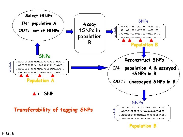
Select t. SNPs OUT: set of t. SNPs Assay t. SNPs in population B SNPs individuals IN: population A individuals … AA CT GT GG TT TT CC GG GG AA GG CT AG CC … Population A … AG ? ? GG ? ? ? CC ? ? ? AG ? ? ? … … AA ? ? GG ? ? ? CG ? ? ? GG ? ? ? … Reconstruct SNPs … AG CT GT GG CT CC CG AG AG AC AG CT … … AG CC GG GT CT CT CC GG AG CC GG CC AG CT … … AG ? ? GG ? ? ? CC ? ? ? AA ? ? ? … Population B SNPs … GG TT TT GG TT CC GG AG AA AC AG CT GG CT … … AA ? ? GT ? ? ? CG ? ? ? AA ? ? ? … IN: population A & assayed t. SNPs in B OUT: unassayed SNPs in B : t. SNP Transferability of tagging SNPs individuals SNPs … AA TT GT TT CC CT CG AG GG CC AA TT … … AG CT GG TT TT CT CC GG AA AA AA CC AA TT … … AG CC GG GT CT CC CC AG AA AC AG CT AA CT … … AA CC GG GT CT TT CG AA AG CC GG CT AG CC … Population B FIG. 6

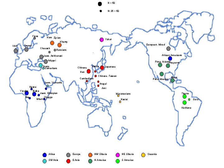
N > 50 N: 25 ~ 50 Finns Kom Zyrian Yakut Khanty Irish European, Mixed Danes Chuvash Russians African Americans Jews, Ashkenazi Adygei Druze Samaritans Pima, Arizona Cheyenne Chinese, Hakka Japanese Han Cambodians Jews, Yemenite Ibo Pima, Mexico Maya Atayal Hausa Yoruba Chinese, Taiwan Ami Biaka Jews, Ethiopian Mbuti Ticuna Micronesians Chagga Nasioi Surui Karitiana Africa Europe NW Siberia NE Siberia SW Asia E Asia N America S America Oceania

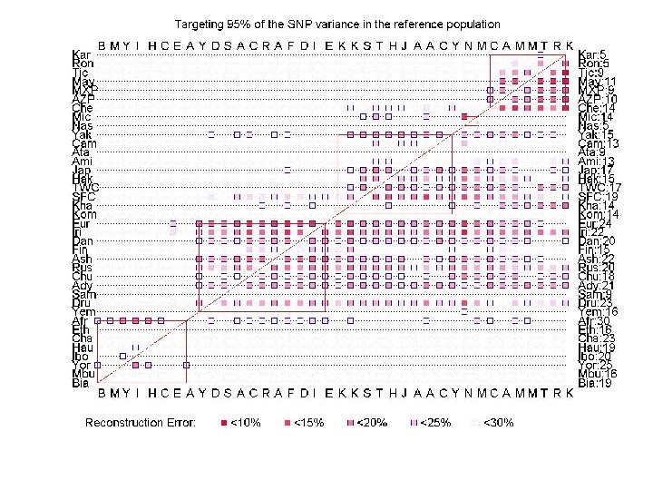
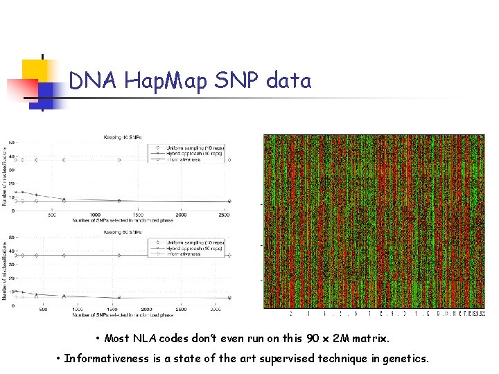
DNA Hap. Map SNP data • Most NLA codes don’t even run on this 90 x 2 M matrix. • Informativeness is a state of the art supervised technique in genetics.

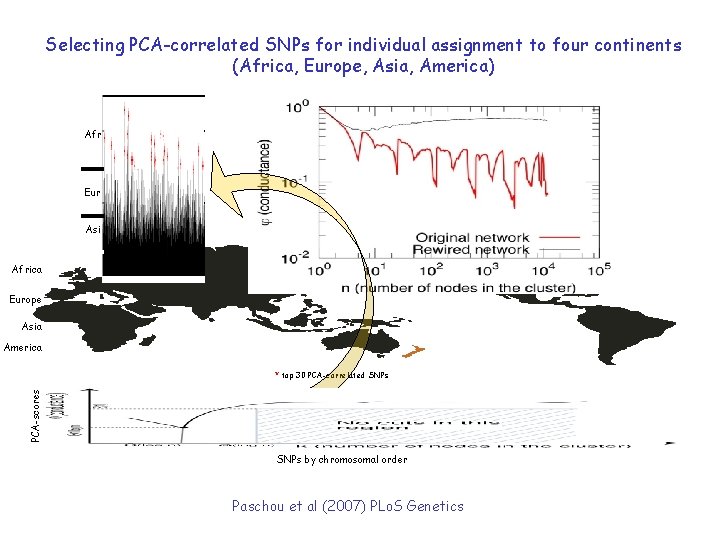
Selecting PCA-correlated SNPs for individual assignment to four continents (Africa, Europe, Asia, America) Afr Eur Asi Africa Ame Europe Asia America PCA-scores * top 30 PCA-correlated SNPs by chromosomal order Paschou et al (2007) PLo. S Genetics

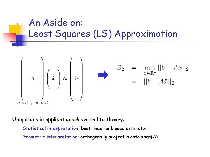
An Aside on: Least Squares (LS) Approximation Ubiquitous in applications & central to theory: Statistical interpretation: best linear unbiased estimator. Geometric interpretation: orthogonally project b onto span(A).

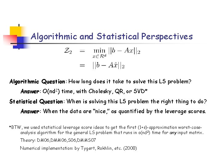
Algorithmic and Statistical Perspectives Algorithmic Question: How long does it take to solve this LS problem? Answer: O(nd 2) time, with Cholesky, QR, or SVD* Statistical Question: When is solving this LS problem the right thing to do? Answer: When the data are “nice, ” as quantified by the leverage scores. *BTW, we used statistical leverage score ideas to get the first (1+ )-approximation worst-caseanalysis algorithm for the general LS problem that runs in o(nd 2) time for any input matrix. Theory: DM 06, DMM 06, S 06, DMMS 07 Numerical implementation: by Tygert, Rokhlin, etc. (2008)

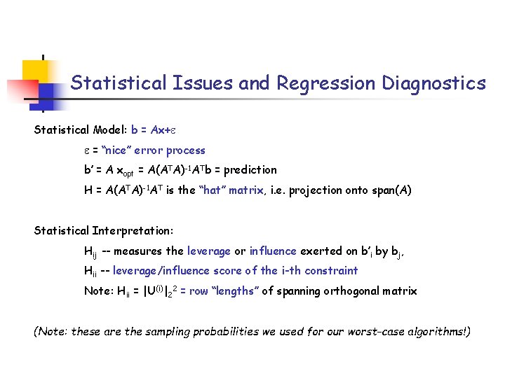
Statistical Issues and Regression Diagnostics Statistical Model: b = Ax+ = “nice” error process b’ = A xopt = A(ATA)-1 ATb = prediction H = A(ATA)-1 AT is the “hat” matrix, i. e. projection onto span(A) Statistical Interpretation: Hij -- measures the leverage or influence exerted on b’i by bj, Hii -- leverage/influence score of the i-th constraint Note: Hii = |U(i)|22 = row “lengths” of spanning orthogonal matrix (Note: these are the sampling probabilities we used for our worst-case algorithms!)

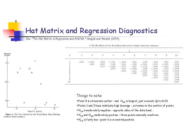
Hat Matrix and Regression Diagnostics See: “The Hat Matrix in Regression and ANOVA, ” Hoaglin and Welsch (1978) Things to note: • Point 4 is a bivariate outlier - and H 4, 4 is largest, just exceeds 2 p/n=6/10. • Points 1 and 3 have relatively high leverage - extremes in the scatter of points. • H 1, 4 is moderately negative - opposite sides of the data band. • H 1, 8 and H 1, 10 moderately positive - those points mutually reinforce. • H 6, 6 is fairly low - point 6 is in central position.

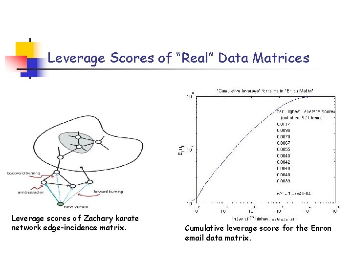
Leverage Scores of “Real” Data Matrices Leverage scores of Zachary karate network edge-incidence matrix. Cumulative leverage score for the Enron email data matrix.

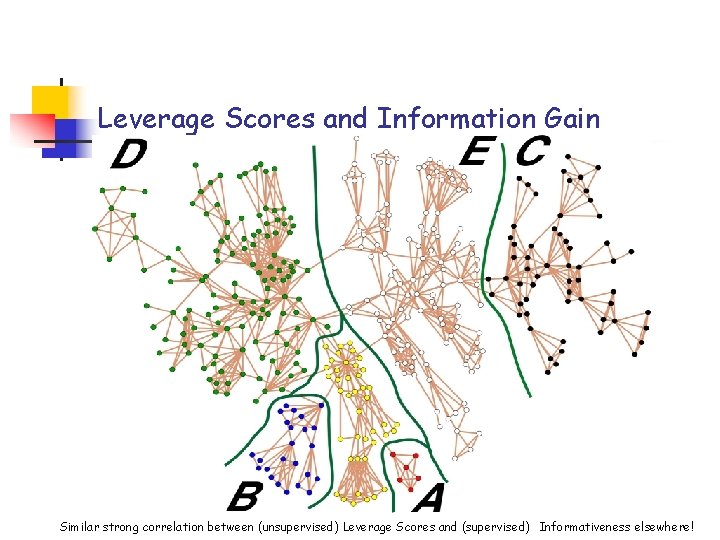
Leverage Scores and Information Gain Similar strong correlation between (unsupervised) Leverage Scores and (supervised) Informativeness elsewhere!

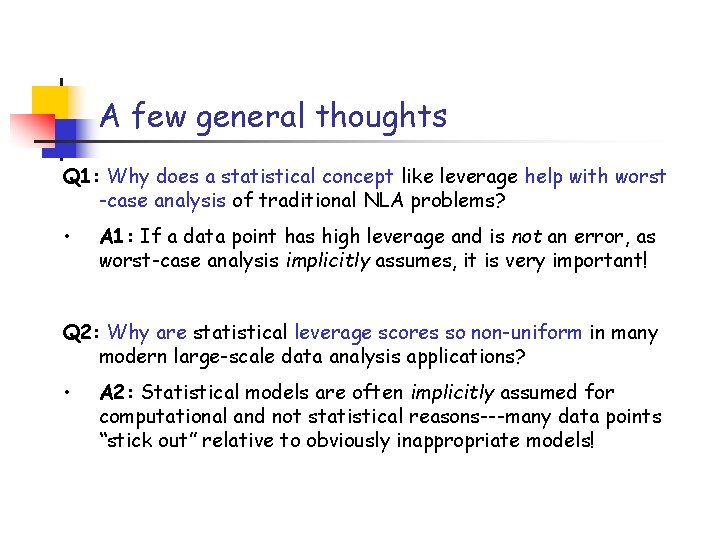
A few general thoughts Q 1: Why does a statistical concept like leverage help with worst -case analysis of traditional NLA problems? • A 1: If a data point has high leverage and is not an error, as worst-case analysis implicitly assumes, it is very important! Q 2: Why are statistical leverage scores so non-uniform in many modern large-scale data analysis applications? • A 2: Statistical models are often implicitly assumed for computational and not statistical reasons---many data points “stick out” relative to obviously inappropriate models!

Outline • “Algorithmic” and “statistical” perspectives on data problems • Genetics application DNA SNP analysis --> choose columns from a matrix • Internet application Community finding --> partitioning a graph In many large-scale data applications, “algorithmic” and “statistical” perspectives interact in fruitful ways --- we use statistical properties implicit in worst-case algorithms to make domain-specific claims!

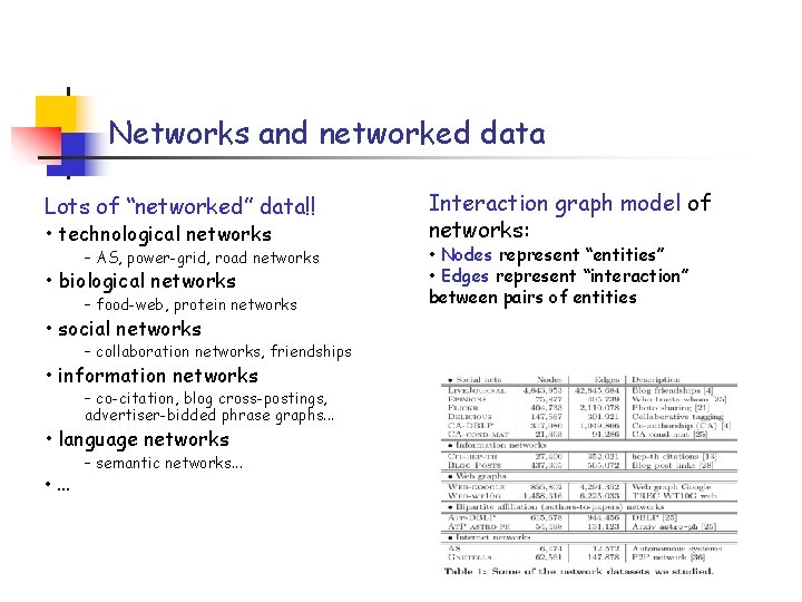
Networks and networked data Lots of “networked” data!! • technological networks – AS, power-grid, road networks • biological networks – food-web, protein networks • social networks – collaboration networks, friendships • information networks – co-citation, blog cross-postings, advertiser-bidded phrase graphs. . . • language networks • . . . – semantic networks. . . Interaction graph model of networks: • Nodes represent “entities” • Edges represent “interaction” between pairs of entities

Social and Information Networks

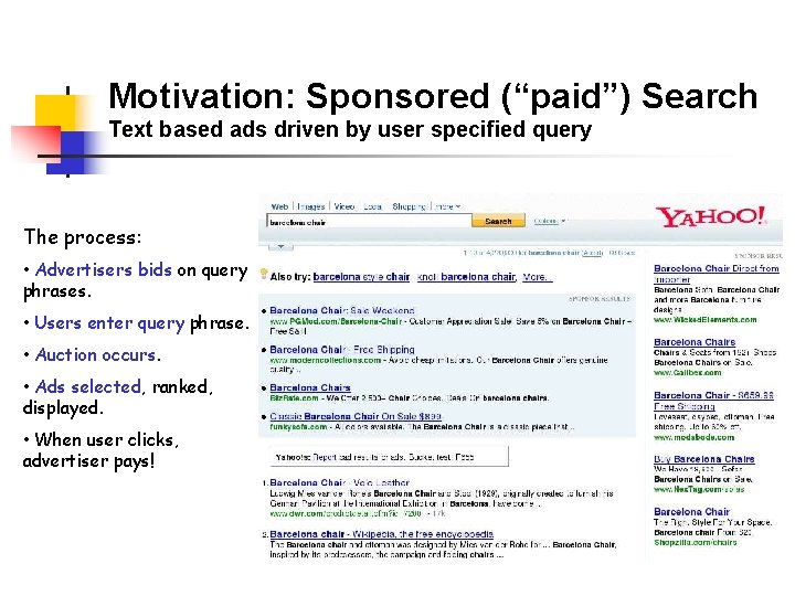
Motivation: Sponsored (“paid”) Search Text based ads driven by user specified query The process: • Advertisers bids on query phrases. • Users enter query phrase. • Auction occurs. • Ads selected, ranked, displayed. • When user clicks, advertiser pays!

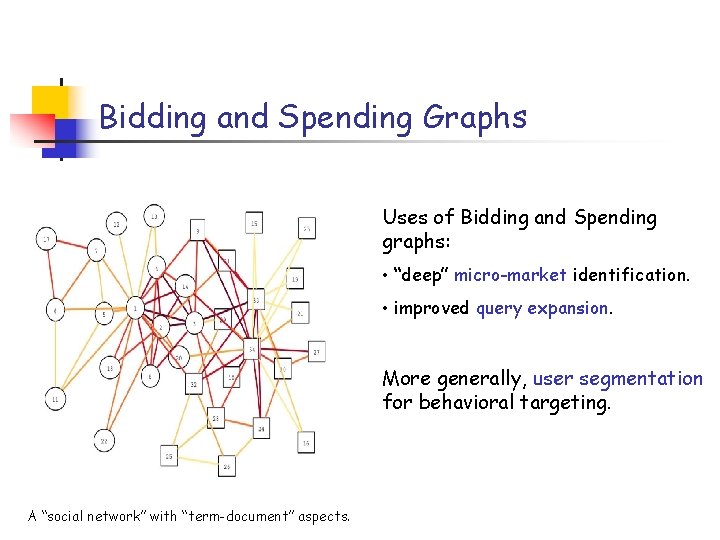
Bidding and Spending Graphs Uses of Bidding and Spending graphs: • “deep” micro-market identification. • improved query expansion. More generally, user segmentation for behavioral targeting. A “social network” with “term-document” aspects.

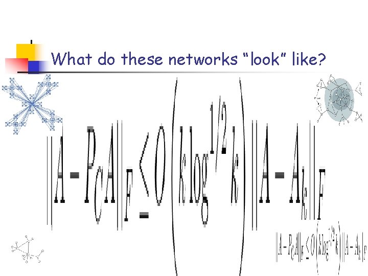
What do these networks “look” like?

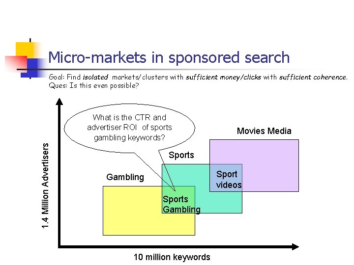
Micro-markets in sponsored search Goal: Find isolated markets/clusters with sufficient money/clicks with sufficient coherence. Ques: Is this even possible? 1. 4 Million Advertisers What is the CTR and advertiser ROI of sports gambling keywords? Movies Media Sports Sport videos Gambling Sports Gambling 10 million keywords

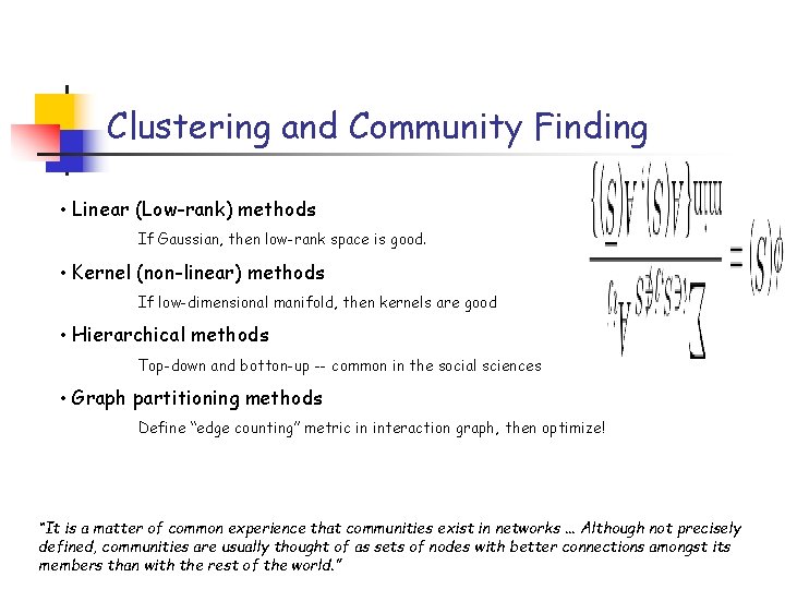
Clustering and Community Finding • Linear (Low-rank) methods If Gaussian, then low-rank space is good. • Kernel (non-linear) methods If low-dimensional manifold, then kernels are good • Hierarchical methods Top-down and botton-up -- common in the social sciences • Graph partitioning methods Define “edge counting” metric in interaction graph, then optimize! “It is a matter of common experience that communities exist in networks. . . Although not precisely defined, communities are usually thought of as sets of nodes with better connections amongst its members than with the rest of the world. ”

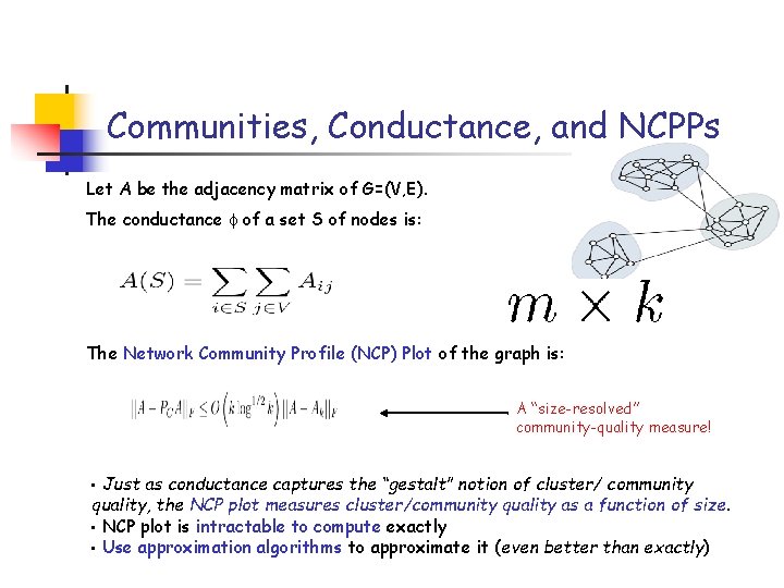
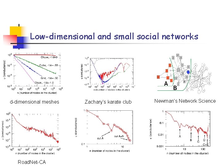
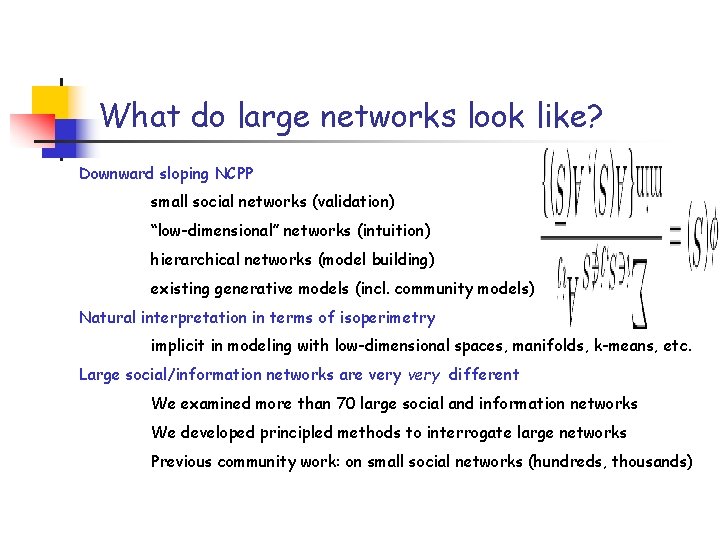
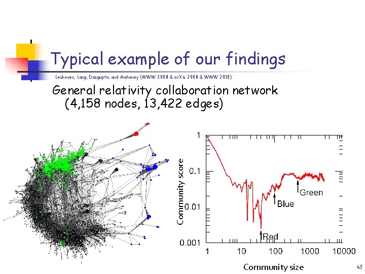
Communities, Conductance, and NCPPs Let A be the adjacency matrix of G=(V, E). The conductance of a set S of nodes is: The Network Community Profile (NCP) Plot of the graph is: A “size-resolved” community-quality measure! Just as conductance captures the “gestalt” notion of cluster/ community quality, the NCP plot measures cluster/community quality as a function of size. • NCP plot is intractable to compute exactly • Use approximation algorithms to approximate it (even better than exactly) •

Probing Large Networks with Approximation Algorithms Idea: Use approximation algorithms for NP-hard graph partitioning problems as experimental probes of network structure. Spectral - (quadratic approx) - confuses “long paths” with “deep cuts” Multi-commodity flow - (log(n) approx) - difficulty with expanders SDP - (sqrt(log(n)) approx) - best in theory Metis - (multi-resolution for mesh-like graphs) - common in practice X+MQI - post-processing step on, e. g. , Spectral of Metis+MQI - best conductance (empirically) Local Spectral - connected and tighter sets (empirically) We are not interested in partitions per se, but in probing network structure.

Approximation algorithms as experimental probes? The usual modus operandi for approximation algorithms: • define an objective, the numerical value of which is intractable to compute • develop approximation algorithm that returns approximation to that number • graph achieving the approximation may be unrelated to the graph achieving the exact optimum. But, for randomized approximation algorithms with a geometric flavor (e. g. matrix algorithms, regression algorithms, eigenvector algorithms; duality algorithms, etc): • often can approximate the vector achieving the exact solution • randomized algorithms compute an ensemble of answers -- the details of which depend on choices made by the algorithm • maybe compare different approximation algorithms for the same problem.

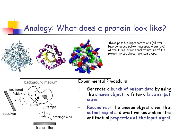
Analogy: What does a protein look like? Three possible representations (all-atom; backbone; and solvent-accessible surface) of the three-dimensional structure of the protein triose phosphate isomerase. Experimental Procedure: • Generate a bunch of output data by using the unseen object to filter a known input signal. • Reconstruct the unseen object given the output signal and what we know about the artifactual properties of the input signal.

Low-dimensional and small social networks d-dimensional meshes Road. Net-CA Zachary’s karate club Newman’s Network Science

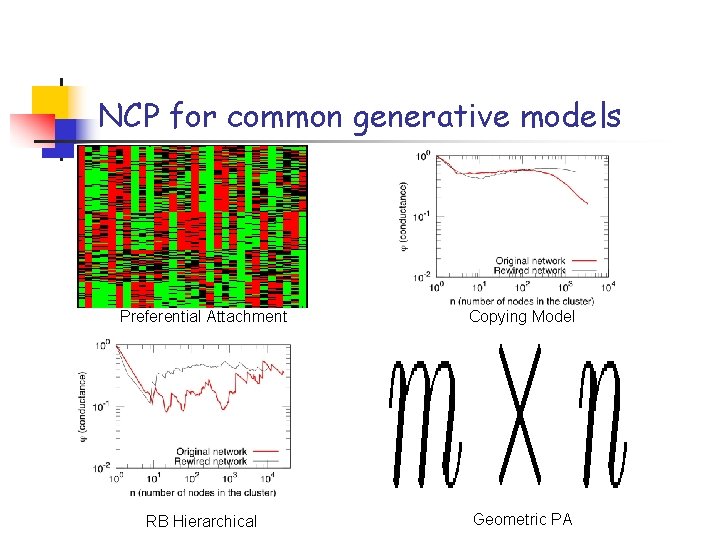
NCP for common generative models Preferential Attachment Copying Model RB Hierarchical Geometric PA

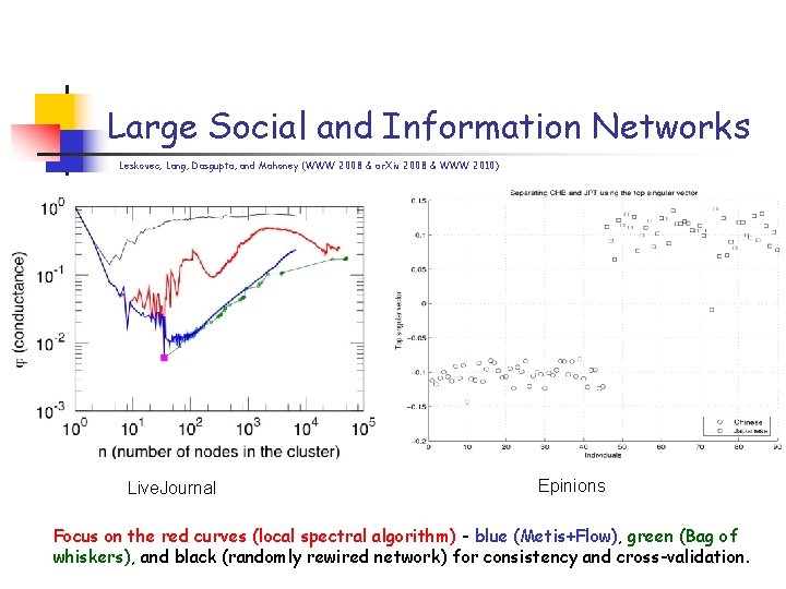
What do large networks look like? Downward sloping NCPP small social networks (validation) “low-dimensional” networks (intuition) hierarchical networks (model building) existing generative models (incl. community models) Natural interpretation in terms of isoperimetry implicit in modeling with low-dimensional spaces, manifolds, k-means, etc. Large social/information networks are very different We examined more than 70 large social and information networks We developed principled methods to interrogate large networks Previous community work: on small social networks (hundreds, thousands)

Typical example of our findings Leskovec, Lang, Dasgupta, and Mahoney (WWW 2008 & ar. Xiv 2008 & WWW 2010) Community score General relativity collaboration network (4, 158 nodes, 13, 422 edges) Community size 45

Large Social and Information Networks Leskovec, Lang, Dasgupta, and Mahoney (WWW 2008 & ar. Xiv 2008 & WWW 2010) Live. Journal Epinions Focus on the red curves (local spectral algorithm) - blue (Metis+Flow), green (Bag of whiskers), and black (randomly rewired network) for consistency and cross-validation.

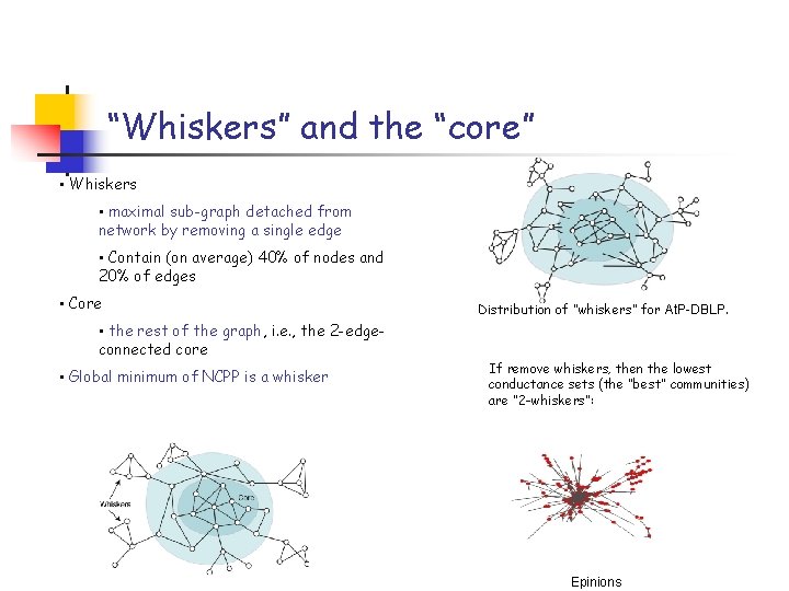
“Whiskers” and the “core” • Whiskers • maximal sub-graph detached from network by removing a single edge • Contain (on average) 40% of nodes and 20% of edges • Core • the rest of the graph, i. e. , the 2 -edgeconnected core • Global minimum of NCPP is a whisker Distribution of “whiskers” for At. P-DBLP. If remove whiskers, then the lowest conductance sets (the “best” communities) are “ 2 -whiskers”: Epinions

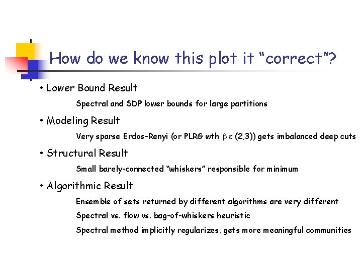
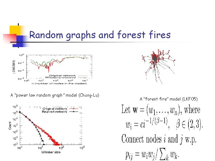
How do we know this plot it “correct”? • Lower Bound Result Spectral and SDP lower bounds for large partitions • Modeling Result Very sparse Erdos-Renyi (or PLRG wth (2, 3)) gets imbalanced deep cuts • Structural Result Small barely-connected “whiskers” responsible for minimum • Algorithmic Result Ensemble of sets returned by different algorithms are very different Spectral vs. flow vs. bag-of-whiskers heuristic Spectral method implicitly regularizes, gets more meaningful communities

Random graphs and forest fires A “power law random graph” model (Chung-Lu) A “forest fire” model (LKF 05)

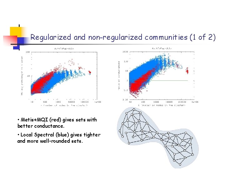
Regularized and non-regularized communities (1 of 2) • Metis+MQI (red) gives sets with better conductance. • Local Spectral (blue) gives tighter and more well-rounded sets.

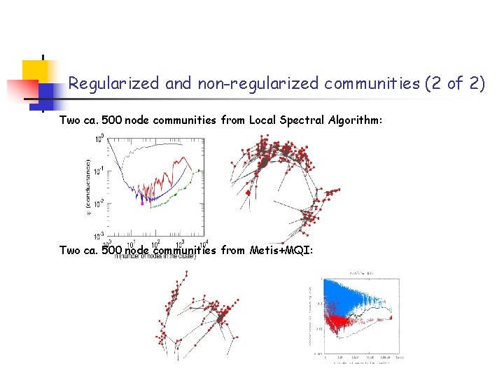
Regularized and non-regularized communities (2 of 2) Two ca. 500 node communities from Local Spectral Algorithm: Two ca. 500 node communities from Metis+MQI:

A few general thoughts Regularization is typically implemented by adding a norm constraint • makes the problem harder (think L 1 -regularized L 2 regression). Approximation algorithms for intractable graph problems implicitly regularize • relative to combinatorial optimum • incorporate empirical signatures of bias-variance tradeoff. Use statistical properties implicit in worst-case algorithms to provide insights into informatics graphs • good since networks are large, sparse, and noisy.

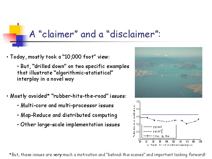
A “claimer” and a “disclaimer”: • Today, mostly took a “ 10, 000 foot” view: • But, “drilled down” on two specific examples that illustrate “algorithmic-statistical” interplay in a novel way • Mostly avoided* “rubber-hits-the-road” issues: • Multi-core and multi-processor issues • Map-Reduce and distributed computing • Other large-scale implementation issues *But, these issues are very much a motivation and “behind-the-scenes” and important looking forward!

Conclusion • “Algorithmic” and “statistical” perspectives on data problems • Genetics application DNA SNP analysis --> choose columns from a matrix • Internet application Community finding --> partitioning a graph In many large-scale data applications, “algorithmic” and “statistical” perspectives interact in fruitful ways.

MMDS Workshop on “Algorithms for Modern Massive Data Sets” (http: //mmds. stanford. edu) at Stanford University, June 15 -18, 2010 Objectives: - Address algorithmic, statistical, and mathematical challenges in modern statistical data analysis. - Explore novel techniques for modeling and analyzing massive, high-dimensional, and nonlinearly-structured data. - Bring together computer scientists, statisticians, mathematicians, and data analysis practitioners to promote cross-fertilization of ideas. Organizers: M. W. Mahoney, P. Drineas, A. Shkolnik, L-H. Lim, and G. Carlsson. Registration will be available soon!