A systematic procedure for economic plantwide control Sigurd

A systematic procedure for economic plantwide control Sigurd Skogestad Department of Chemical Engineering Norwegian University of Science and Tecnology (NTNU) Trondheim, Norway 1 Lund, 29 Sept. 2016

Outline • • Our paradigm basaed on time scale separation Plantwide control procedure based on economics Example: Runner Selection of primary controlled variables (CV 1=H y) – Optimal is gradient, CV 1=Ju with setpoint=0 – General CV 1=Hy. Nullspace and exact local method This is the truth and the only truth • Throughput manipulator (TPM) location • Examples • Conclusion 2

How we design a control system for a complete chemical plant? • • 5 Where do we start? What should we control? and why? etc.

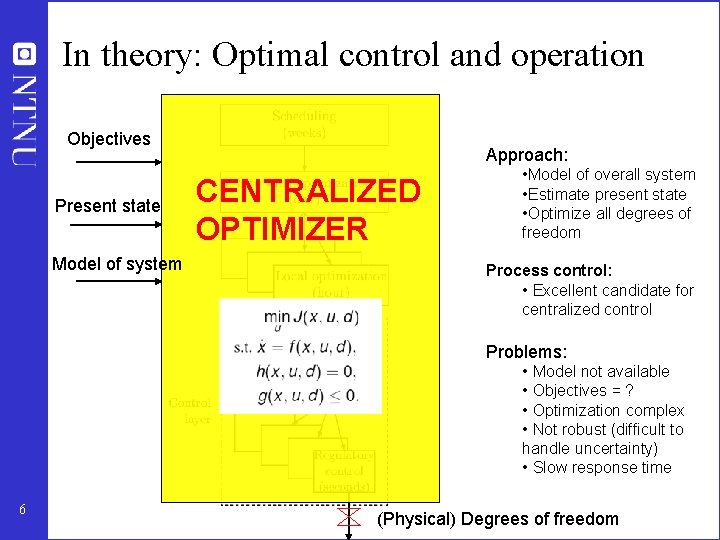
In theory: Optimal control and operation Objectives Present state Model of system Approach: CENTRALIZED OPTIMIZER • Model of overall system • Estimate present state • Optimize all degrees of freedom Process control: • Excellent candidate for centralized control Problems: • Model not available • Objectives = ? • Optimization complex • Not robust (difficult to handle uncertainty) • Slow response time 6 (Physical) Degrees of freedom

Practice: Engineering systems • Most (all? ) large-scale engineering systems are controlled using hierarchies of quite simple controllers – Large-scale chemical plant (refinery) – Commercial aircraft • 100’s of loops • Simple components: PI-control + selectors + cascade + nonlinear fixes + some feedforward Same in biological systems But: Not well understood 7

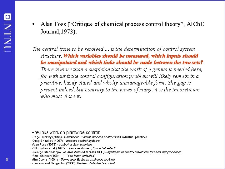
• Alan Foss (“Critique of chemical process control theory”, AICh. E Journal, 1973): The central issue to be resolved. . . is the determination of control system structure. Which variables should be measured, which inputs should be manipulated and which links should be made between the two sets? There is more than a suspicion that the work of a genius is needed here, for without it the control configuration problem will likely remain in a primitive, hazily stated and wholly unmanageable form. The gap is present indeed, but contrary to the views of many, it is theoretician who must close it. Previous work on plantwide control: 8 • Page Buckley (1964) - Chapter on “Overall process control” (still industrial practice) • Greg Shinskey (1967) – process control systems • Alan Foss (1973) - control system structure • Bill Luyben et al. (1975 - ) – case studies ; “snowball effect” • George Stephanopoulos and Manfred Morari (1980) – synthesis of control structures for chemical processes • Ruel Shinnar (1981 - ) - “dominant variables” • Jim Downs (1991) - Tennessee Eastman challenge problem • Larsson and Skogestad (2000): Review of plantwide control

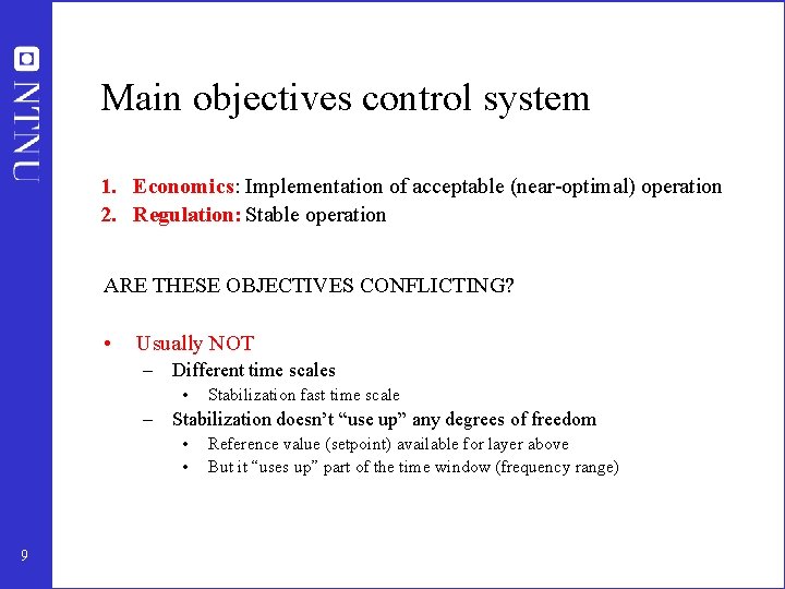
Main objectives control system 1. Economics: Implementation of acceptable (near-optimal) operation 2. Regulation: Stable operation ARE THESE OBJECTIVES CONFLICTING? • Usually NOT – Different time scales • Stabilization fast time scale – Stabilization doesn’t “use up” any degrees of freedom • • 9 Reference value (setpoint) available for layer above But it “uses up” part of the time window (frequency range)

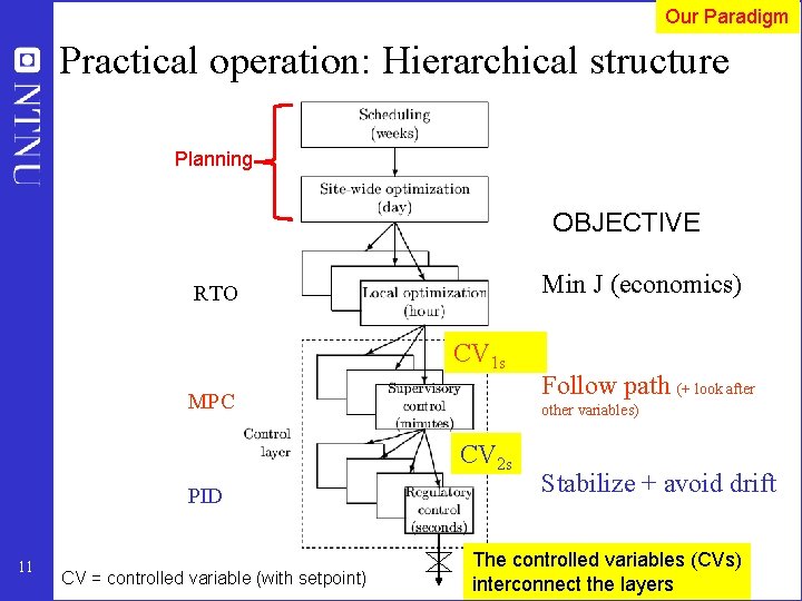
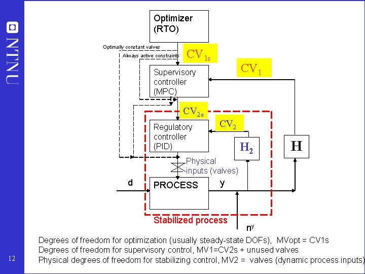
Our Paradigm Practical operation: Hierarchical structure Planning OBJECTIVE Min J (economics) RTO CV 1 s MPC other variables) CV 2 s PID 11 CV = controlled variable (with setpoint) Follow path (+ look after Stabilize + avoid drift u (valves) The controlled variables (CVs) interconnect the layers

Optimizer (RTO) Optimally constant valves Always active constraints CV 1 Supervisory controller (MPC) CV 2 s Regulatory controller (PID) CV 2 H Physical inputs (valves) d PROCESS y Stabilized process 12 ny Degrees of freedom for optimization (usually steady-state DOFs), MVopt = CV 1 s Degrees of freedom for supervisory control, MV 1=CV 2 s + unused valves Physical degrees of freedom for stabilizing control, MV 2 = valves (dynamic process inputs)

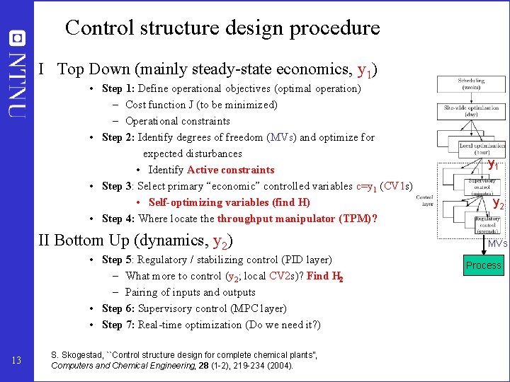
Control structure design procedure I Top Down (mainly steady-state economics, y 1) • Step 1: Define operational objectives (optimal operation) – Cost function J (to be minimized) – Operational constraints • Step 2: Identify degrees of freedom (MVs) and optimize for expected disturbances • Identify Active constraints • Step 3: Select primary “economic” controlled variables c=y 1 (CV 1 s) • Self-optimizing variables (find H) • Step 4: Where locate throughput manipulator (TPM)? II Bottom Up (dynamics, y 2) • Step 5: Regulatory / stabilizing control (PID layer) – What more to control (y 2; local CV 2 s)? Find H 2 – Pairing of inputs and outputs • Step 6: Supervisory control (MPC layer) • Step 7: Real-time optimization (Do we need it? ) 13 S. Skogestad, ``Control structure design for complete chemical plants'', Computers and Chemical Engineering, 28 (1 -2), 219 -234 (2004). y 1 y 2 MVs Process

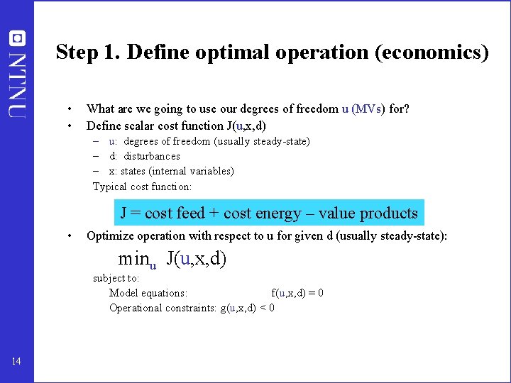
Step 1. Define optimal operation (economics) • • What are we going to use our degrees of freedom u (MVs) for? Define scalar cost function J(u, x, d) – u: degrees of freedom (usually steady-state) – d: disturbances – x: states (internal variables) Typical cost function: J = cost feed + cost energy – value products • Optimize operation with respect to u for given d (usually steady-state): minu J(u, x, d) subject to: Model equations: f(u, x, d) = 0 Operational constraints: g(u, x, d) < 0 14

Step S 2. Optimize (a) Identify degrees of freedom (b) Optimize for expected disturbances • • 15 Need good model, usually steady-state Optimization is time consuming! But it is offline Main goal: Identify ACTIVE CONSTRAINTS A good engineer can often guess the active constraints

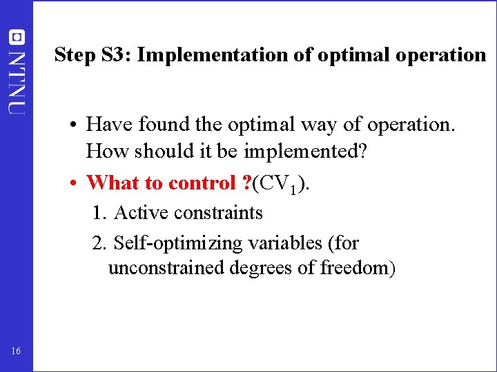
Step S 3: Implementation of optimal operation • Have found the optimal way of operation. How should it be implemented? • What to control ? (CV 1). 1. Active constraints 2. Self-optimizing variables (for unconstrained degrees of freedom) 16

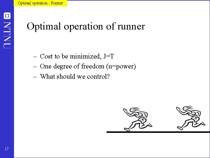
Optimal operation - Runner Optimal operation of runner – Cost to be minimized, J=T – One degree of freedom (u=power) – What should we control? 17

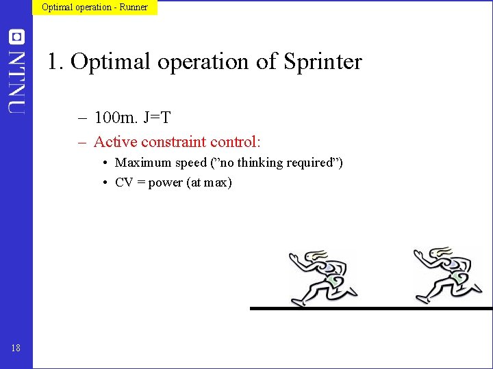
Optimal operation - Runner 1. Optimal operation of Sprinter – 100 m. J=T – Active constraint control: • Maximum speed (”no thinking required”) • CV = power (at max) 18

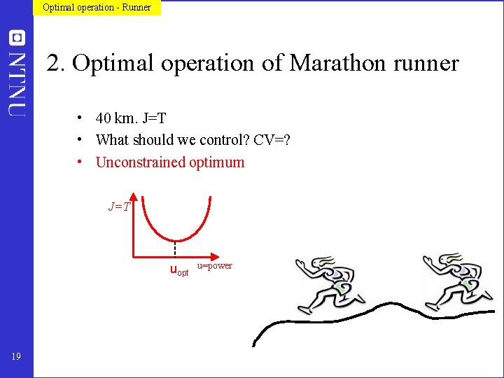
Optimal operation - Runner 2. Optimal operation of Marathon runner • 40 km. J=T • What should we control? CV=? • Unconstrained optimum J=T uopt 19 u=power

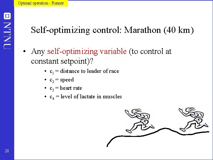
Optimal operation - Runner Self-optimizing control: Marathon (40 km) • Any self-optimizing variable (to control at constant setpoint)? • • 20 c 1 = distance to leader of race c 2 = speed c 3 = heart rate c 4 = level of lactate in muscles

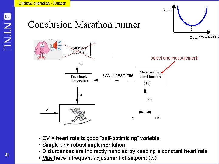
Optimal operation - Runner J=T Conclusion Marathon runner copt c=heart rate select one measurement CV 1 = heart rate 21 • CV = heart rate is good “self-optimizing” variable • Simple and robust implementation • Disturbances are indirectly handled by keeping a constant heart rate • May have infrequent adjustment of setpoint (cs)

Summary Step 3. What should we control (CV 1)? Selection of primary controlled variables c = CV 1 1. Control active constraints! 2. Unconstrained variables: Control self-optimizing variables! • Old idea (Morari et al. , 1980): “We want to find a function c of the process variables which when held constant, leads automatically to the optimal adjustments of the manipulated variables, and with it, the optimal operating conditions. ” 22

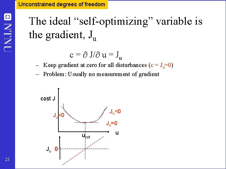
Unconstrained degrees of freedom The ideal “self-optimizing” variable is the gradient, Ju c = J/ u = Ju – Keep gradient at zero for all disturbances (c = Ju=0) – Problem: Usually no measurement of gradient cost J Ju<0 Ju=0 uopt u Ju 0 23

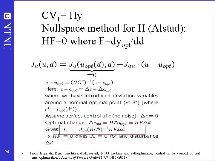
CV 1= Hy Nullspace method for H (Alstad): HF=0 where F=dyopt/dd 26 • Proof. Appendix B in: Jäschke and Skogestad, ”NCO tracking and self-optimizing control in the context of real -time optimization”, Journal of Process Control, 1407 -1416 (2011)

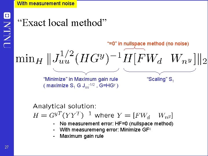
With measurement noise “Exact local method” “=0” in nullspace method (no noise) “Minimize” in Maximum gain rule ( maximize S 1 G Juu-1/2 , G=HGy ) “Scaling” S 1 - No measurement error: HF=0 (nullspace method) - With measuremeng error: Minimize GFc - Maximum gain rule 27

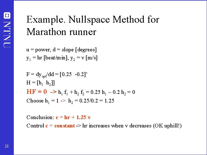
Example. Nullspace Method for Marathon runner u = power, d = slope [degrees] y 1 = hr [beat/min], y 2 = v [m/s] F = dyopt/dd = [0. 25 -0. 2]’ H = [h 1 h 2]] HF = 0 -> h 1 f 1 + h 2 f 2 = 0. 25 h 1 – 0. 2 h 2 = 0 Choose h 1 = 1 -> h 2 = 0. 25/0. 2 = 1. 25 Conclusion: c = hr + 1. 25 v Control c = constant -> hr increases when v decreases (OK uphill!) 28

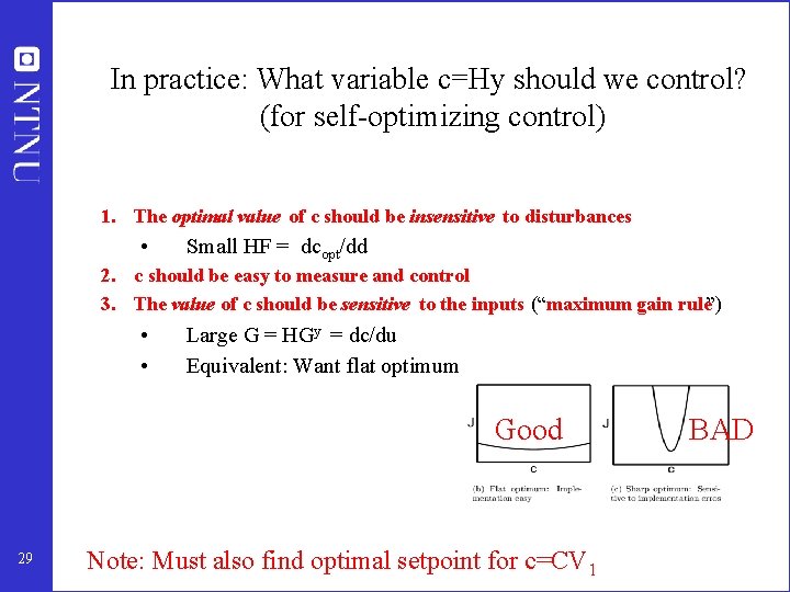
In practice: What variable c=Hy should we control? (for self-optimizing control) 1. The optimal value of c should be insensitive to disturbances • Small HF = dcopt/dd 2. c should be easy to measure and control 3. The value of c should be sensitive to the inputs (“maximum gain rule”) • • 29 Large G = HGy = dc/du Equivalent: Want flat optimum Good Note: Must also find optimal setpoint for c=CV 1 BAD

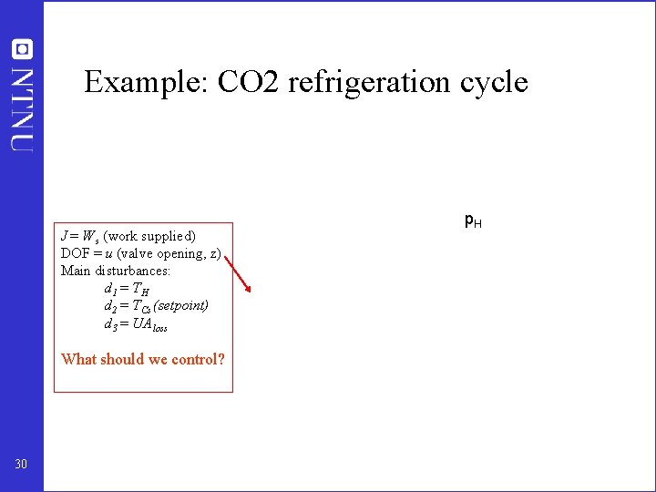
Example: CO 2 refrigeration cycle J = W s (work supplied) DOF = u (valve opening, z) Main disturbances: d 1 = T H d 2 = T Cs (setpoint) d 3 = UA loss p. H What should we control? 30

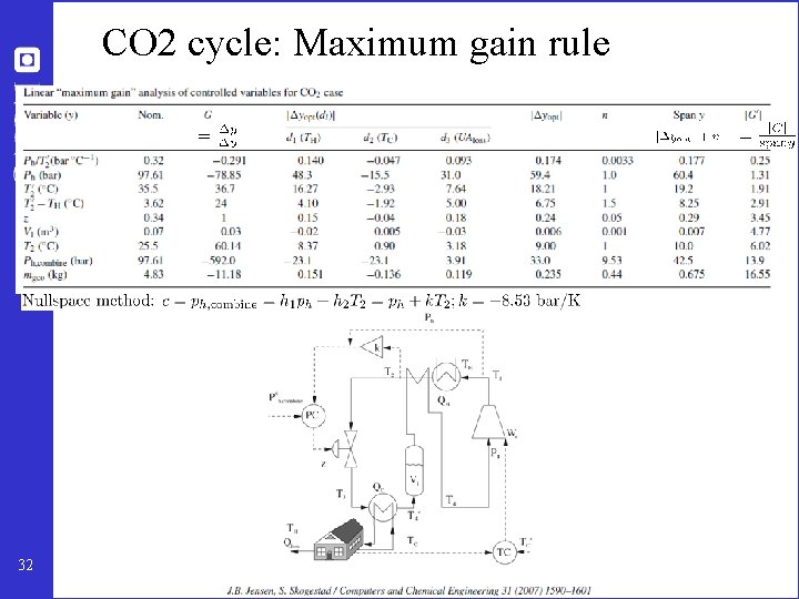
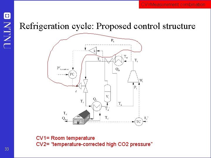
CO 2 refrigeration cycle Step 1. One (remaining) degree of freedom (u=z) Step 2. Objective function. J = Ws (compressor work) Step 3. Optimize operation for disturbances (d 1=TC, d 2=TH, d 3=UA) • Optimum always unconstrained Step 4. Implementation of optimal operation • No good single measurements (all give large losses): – ph, Th, z, … • Nullspace method: Need to combine nu+nd=1+3=4 measurements to have zero disturbance loss • Simpler: Try combining two measurements. Exact local method: – c = h 1 ph + h 2 Th = ph + k Th; k = -8. 53 bar/K • Nonlinear evaluation of loss: OK! 31

CO 2 cycle: Maximum gain rule 32

CV=Measurement combination Refrigeration cycle: Proposed control structure 33 CV 1= Room temperature CV 2= “temperature-corrected high CO 2 pressure”

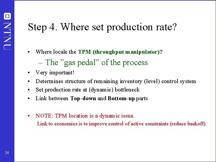
Step 4. Where set production rate? • Where locale the TPM (throughput manipulator)? – The ”gas pedal” of the process • • Very important! Determines structure of remaining inventory (level) control system Set production rate at (dynamic) bottleneck Link between Top-down and Bottom-up parts • NOTE: TPM location is a dynamic issue. Link to economics is to improve control of active constraints (reduce backoff) 34

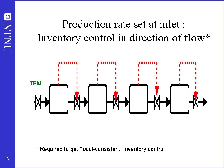
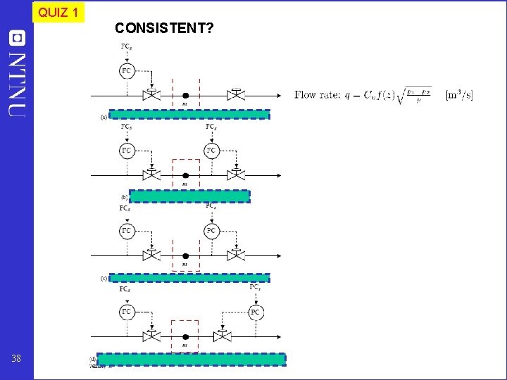
Production rate set at inlet : Inventory control in direction of flow* TPM * Required to get “local-consistent” inventory control 35

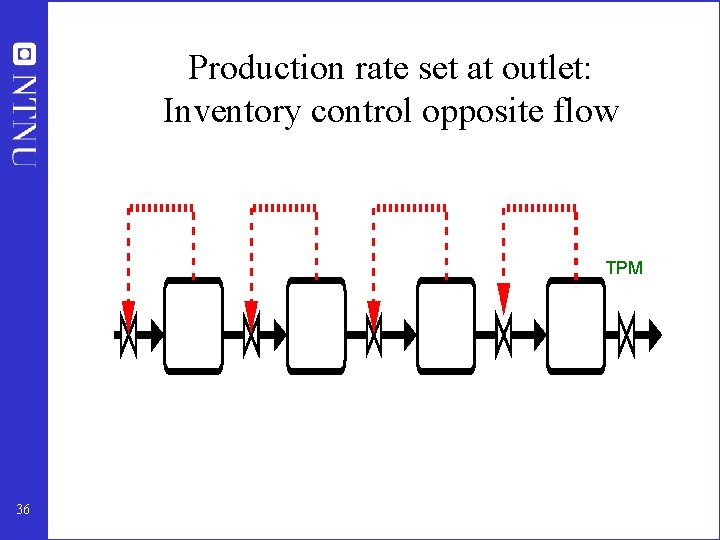
Production rate set at outlet: Inventory control opposite flow TPM 36

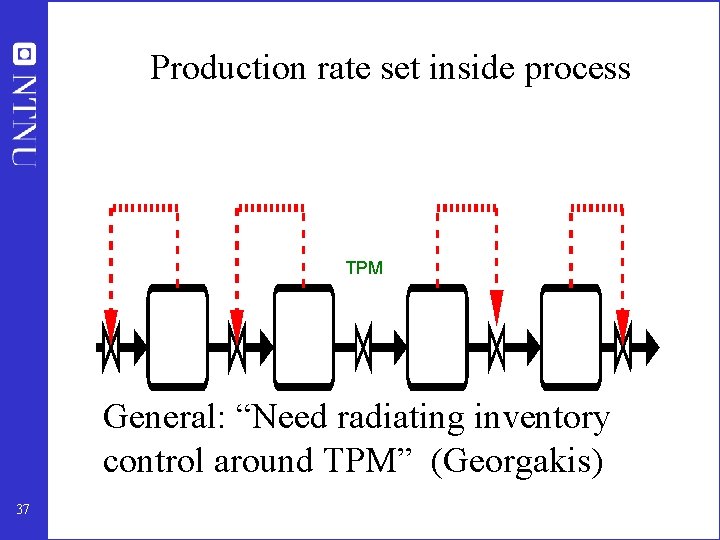
Production rate set inside process TPM General: “Need radiating inventory control around TPM” (Georgakis) 37

QUIZ 1 CONSISTENT? 38

Academic process control community fish pond Optimal centralized Solution (EMPC) Sigurd 44

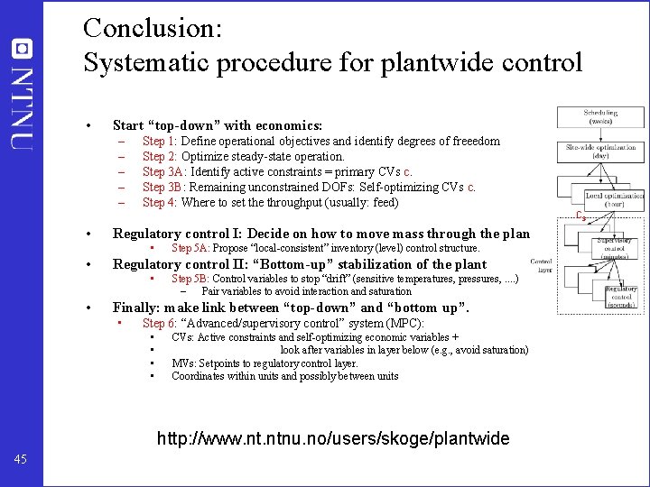
Conclusion: Systematic procedure for plantwide control • Start “top-down” with economics: – – – • Step 1: Define operational objectives and identify degrees of freeedom Step 2: Optimize steady-state operation. Step 3 A: Identify active constraints = primary CVs c. Step 3 B: Remaining unconstrained DOFs: Self-optimizing CVs c. Step 4: Where to set the throughput (usually: feed) Regulatory control I: Decide on how to move mass through the plant: • • Step 5 A: Propose “local-consistent” inventory (level) control structure. Regulatory control II: “Bottom-up” stabilization of the plant • • cs Step 5 B: Control variables to stop “drift” (sensitive temperatures, pressures, . . ) – Pair variables to avoid interaction and saturation Finally: make link between “top-down” and “bottom up”. • Step 6: “Advanced/supervisory control” system (MPC): • • CVs: Active constraints and self-optimizing economic variables + look after variables in layer below (e. g. , avoid saturation) MVs: Setpoints to regulatory control layer. Coordinates within units and possibly between units http: //www. ntnu. no/users/skoge/plantwide 45

Summary and references • The following paper summarizes the procedure: – S. Skogestad, ``Control structure design for complete chemical plants'', Computers and Chemical Engineering, 28 (1 -2), 219 -234 (2004). • There are many approaches to plantwide control as discussed in the following review paper: – T. Larsson and S. Skogestad, ``Plantwide control: A review and a new design procedure'' Modeling, Identification and Control, 21, 209 -240 (2000). • The following paper updates the procedure: – S. Skogestad, ``Economic plantwide control’’, Book chapter in V. Kariwala and V. P. Rangaiah (Eds), Plant-Wide Control: Recent Developments and Applications”, Wiley (2012). • Another paper: – S. Skogestad “Plantwide control: the search for the self-optimizing control structure‘”, J. Proc. Control, 10, 487 -507 (2000). • More information: http: //www. ntnu. no/users/skoge/plantwide 46