503 Applied Macroeconomics Chapter 2 The Solow Growth

503 Applied Macroeconomics Chapter 2. The Solow Growth Model Prof. M. El-Sakka Dept of Economics - Kuwait University

• SOME BASIC FACTS ABOUT GROWTH • 1. High levels of living standards: in industrialized countries, in US 10 times, in Europe 30 times higher than 1 century ago. 50 times and 300 times respectively than 2 centuries ago. • 2. Enormous differences in standards of living, e. g. , US, Germany and Japan are 20 times Bangladesh. • 3. Growth Miracles: the cases where growth exceeds the world average for extended periods, and moves rapidly up the world income distribution. Examples are Japan, South Korea, China. . etc. Average NIC’s growth is over 5% since 1960 s.

• 4. Growth Disasters: the case where growth is less than world levels, e. g. , Argentina (income was behind world leaders in 1900, now in middle income countries), and Sub-Saharan countries (average incomes near subsistence levels). • Implications: vast differences are in nutrition, literacy, infant mortality, life expectancy and, other indicators. • The principal conclusion of the Solow model is that the accumulation of physical capital cannot account for either the vast growth in average output over time or the vast geographic differences in average output. • To address the central questions of growth theory, we must move beyond the Solow model

The Solow model • The Solow model focuses on four variables: output (Y ), capital (K), labor (L), and “knowledge” or the “effectiveness of labor” (A). • Production Function: • Y(t) = F (K(t), A(t)L(t)), (1. 1) • Notice also that A and L enter multiplicatively, known as laboraugmenting or Harrod-neutral, or effective labor.

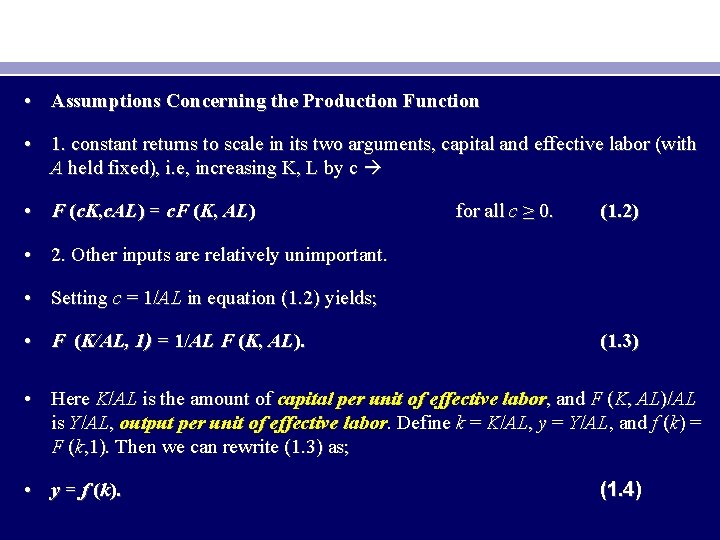
• Assumptions Concerning the Production Function • 1. constant returns to scale in its two arguments, capital and effective labor (with A held fixed), i. e, increasing K, L by c • F (c. K, c. AL) = c. F (K, AL) for all c ≥ 0. (1. 2) • 2. Other inputs are relatively unimportant. • Setting c = 1/AL in equation (1. 2) yields; • F (K/AL, 1) = 1/AL F (K, AL). (1. 3) • Here K/AL is the amount of capital per unit of effective labor, and F (K, AL)/AL is Y/AL, output per unit of effective labor. Define k = K/AL, y = Y/AL, and f (k) = F (k, 1). Then we can rewrite (1. 3) as; • y = f (k). (1. 4)

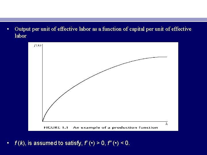
• Output per unit of effective labor as a function of capital per unit of effective labor • f (k), is assumed to satisfy, f’ ( • ) > 0, f” ( • ) < 0.

• the assumptions that f’ (k) is positive and f” (k) is negative imply that the marginal product of capital is positive, but that it declines as capital (per unit of effective labor) rises. • A specific example of a production function is the Cobb–Douglas function, • F (K, AL) = Kα (AL)1−α, • Multiplying both inputs by c gives us; • F (c. K, c. AL) = (c. K )α(c. AL)1−α • = cαc 1−αKα(AL)1−α • = c. F (K, AL). 0< α < 1. (1. 5)

The intensive form; • divide both inputs by AL; this yields • f (k) ≡ F (K/AL, 1) = (K /AL)α = kα. (1. 7) • Equation (1. 7) implies that f’ (k) = αkα− 1. this expression is positive, that it approaches infinity as k approaches zero, and that it approaches zero as k approaches infinity. Finally, • f” (k) = −(1 − α)αkα− 2, which is negative

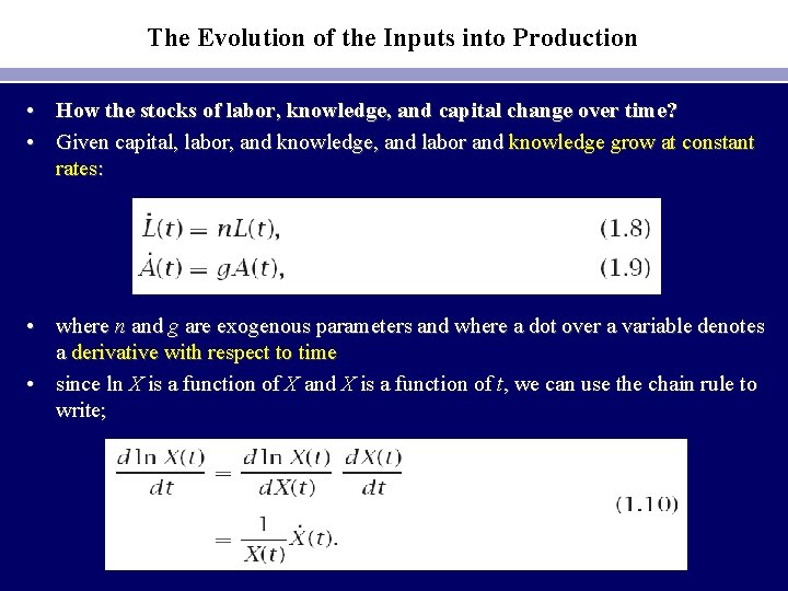
The Evolution of the Inputs into Production • How the stocks of labor, knowledge, and capital change over time? • Given capital, labor, and knowledge, and labor and knowledge grow at constant rates: • where n and g are exogenous parameters and where a dot over a variable denotes a derivative with respect to time • since ln X is a function of X and X is a function of t, we can use the chain rule to write;

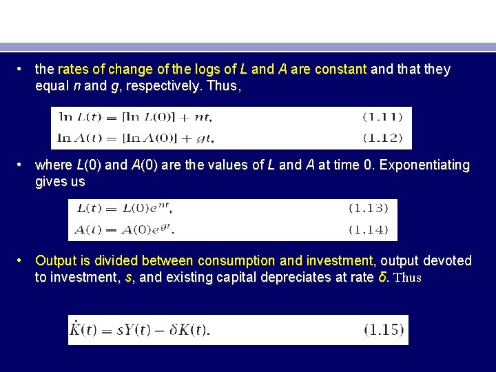
• the rates of change of the logs of L and A are constant and that they equal n and g, respectively. Thus, • where L(0) and A(0) are the values of L and A at time 0. Exponentiating gives us • Output is divided between consumption and investment, output devoted to investment, s, and existing capital depreciates at rate δ. Thus

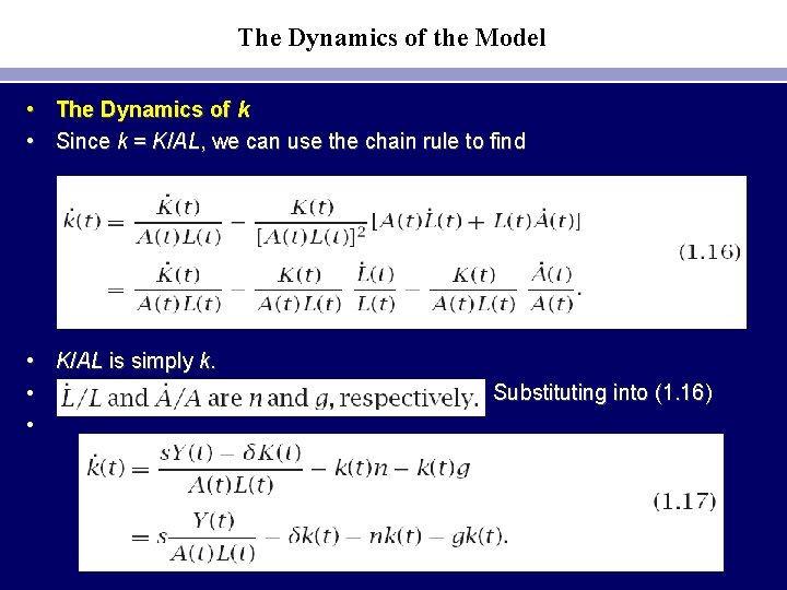
The Dynamics of the Model • The Dynamics of k • Since k = K/AL, we can use the chain rule to find • K/AL is simply k. • • Substituting into (1. 16)

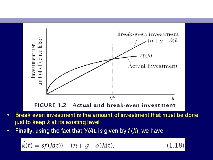
• Break even investment is the amount of investment that must be done just to keep k at its existing level • Finally, using the fact that Y/AL is given by f (k), we have

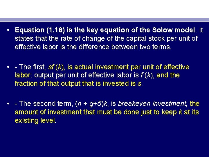
• Equation (1. 18) is the key equation of the Solow model. It states that the rate of change of the capital stock per unit of effective labor is the difference between two terms. • - The first, sf (k), is actual investment per unit of effective labor: output per unit of effective labor is f (k), and the fraction of that output that is invested is s. • - The second term, (n + g+δ)k, is breakeven investment, the amount of investment that must be done just to keep k at its existing level.

• Two reasons that some investment is needed to prevent k from falling (break even). • First, existing capital is depreciating. δk term in (1. 18). • Second, since the quantity of effective labor is growing at rate n + g, the capital stock must grow at rate n + g to hold k steady. This is the (n + g)k term in (1. 18). Note that: • When sf (k) exceeds (n + g+δ)k, , k is rising. • When sf (k) falls short of (n + g+δ)k, k is falling. • And when the two are equal, k is constant.

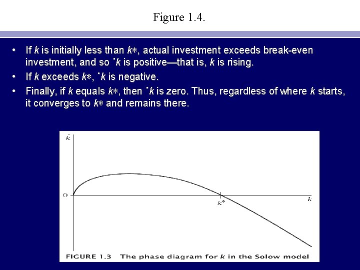
Figure 1. 4. • If k is initially less than k∗, actual investment exceeds break-even investment, and so ˙k is positive—that is, k is rising. • If k exceeds k∗, ˙k is negative. • Finally, if k equals k∗, then ˙k is zero. Thus, regardless of where k starts, it converges to k∗ and remains there.

• The Balanced Growth Path • the Solow model implies that, the economy converges to a balanced growth path—a situation where each variable of the model is growing at a constant rate. • On the balanced growth path, the growth rate of output per worker is determined solely by the rate of technological progress.

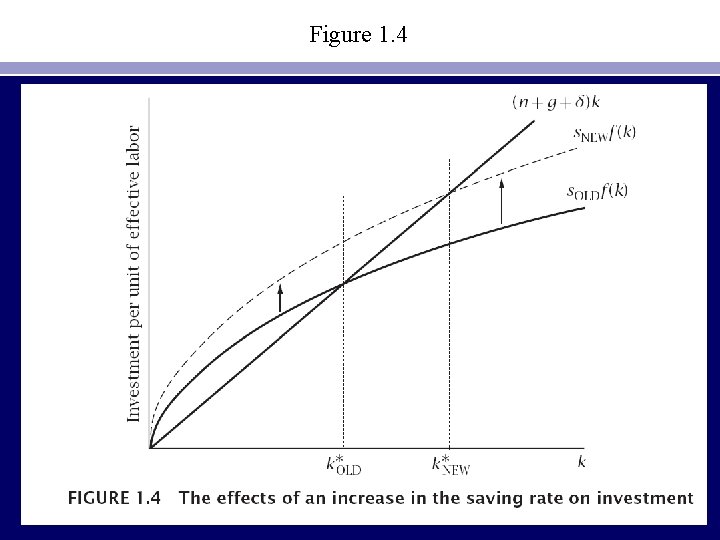
• The Impact of a Change in the Saving Rate • suppose that there is a permanent increase in s. • The Impact on Output • ↑ s shifts the actual investment line up, and so k∗ ↑. This is shown in Figure 1. 4. At this level, actual investment now exceeds break-even investment and so ˙k is positive. Thus k begins to rise until it reaches the new value of k∗

Figure 1. 4

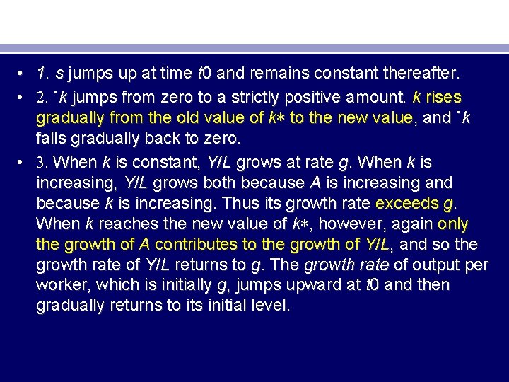
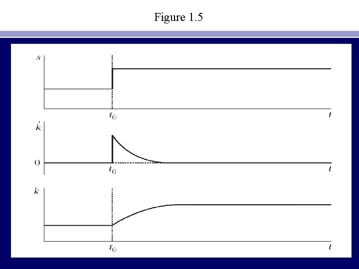
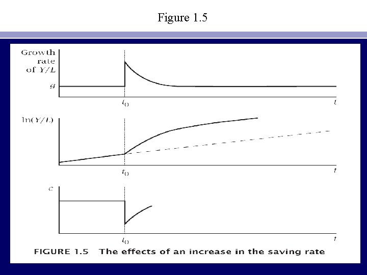
• 1. s jumps up at time t 0 and remains constant thereafter. • 2. ˙k jumps from zero to a strictly positive amount. k rises gradually from the old value of k∗ to the new value, and ˙k falls gradually back to zero. • 3. When k is constant, Y/L grows at rate g. When k is increasing, Y/L grows both because A is increasing and because k is increasing. Thus its growth rate exceeds g. When k reaches the new value of k∗, however, again only the growth of A contributes to the growth of Y/L, and so the growth rate of Y/L returns to g. The growth rate of output per worker, which is initially g, jumps upward at t 0 and then gradually returns to its initial level.

Figure 1. 5

Figure 1. 5

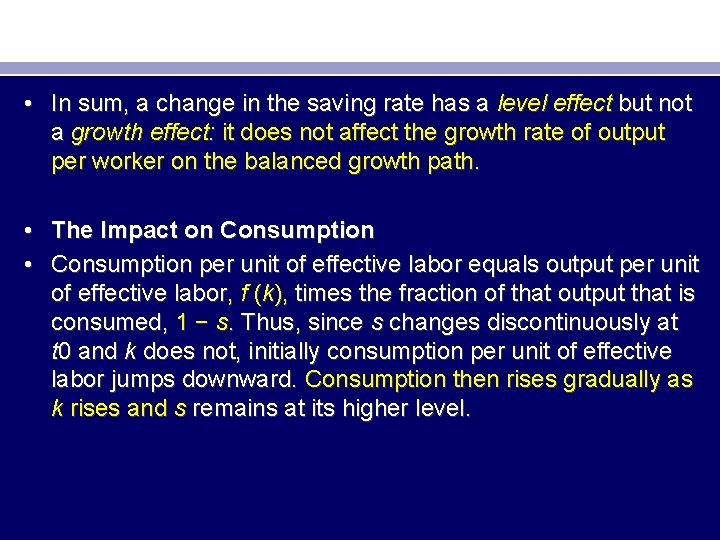
• In sum, a change in the saving rate has a level effect but not a growth effect: it does not affect the growth rate of output per worker on the balanced growth path. • The Impact on Consumption • Consumption per unit of effective labor equals output per unit of effective labor, f (k), times the fraction of that output that is consumed, 1 − s. Thus, since s changes discontinuously at t 0 and k does not, initially consumption per unit of effective labor jumps downward. Consumption then rises gradually as k rises and s remains at its higher level.

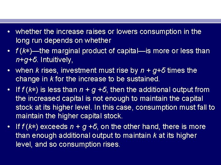
• whether the increase raises or lowers consumption in the long run depends on whether • f (k∗)—the marginal product of capital—is more or less than n+g+δ. Intuitively, • when k rises, investment must rise by n + g+δ times the change in k for the increase to be sustained. • If f (k∗) is less than n + g +δ, then the additional output from the increased capital is not enough to maintain the capital stock at its higher level. In this case, consumption must fall to maintain the higher capital stock. • If f (k∗) exceeds n + g +δ, on the other hand, there is more than enough additional output to maintain k at its higher level, and so consumption rises.

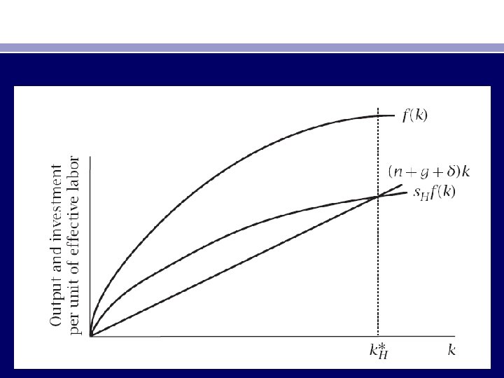
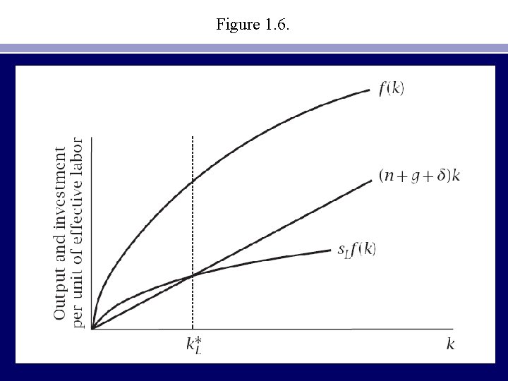
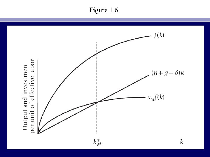
Figure 1. 6. • c ∗ is the distance between f (k) and (n+g+δ)k at k = k∗. Figure 1. 6 shows the determinants of c ∗ for three different values of s (and hence three different values of k∗). • In the top panel, s is high, and so k∗ is high and f (k∗) is less than n + g + δ. As a result, an increase in the saving rate lowers consumption even when the economy has reached its new balanced growth path. • In the middle panel, s is low, k∗ is low, f (k∗) is greater than n + g + δ, and an increase in s raises consumption in the long run. • In the bottom panel, s is at the level that causes f (k∗) to just equal n + g+δ—that is, the f (k) and (n + g+δ)k loci are parallel at k =k∗. In this case, a marginal change in s has no effect on consumption in the long run, and consumption is at its maximum possible level among balanced growth paths.

Figure 1. 6.

Figure 1. 6.

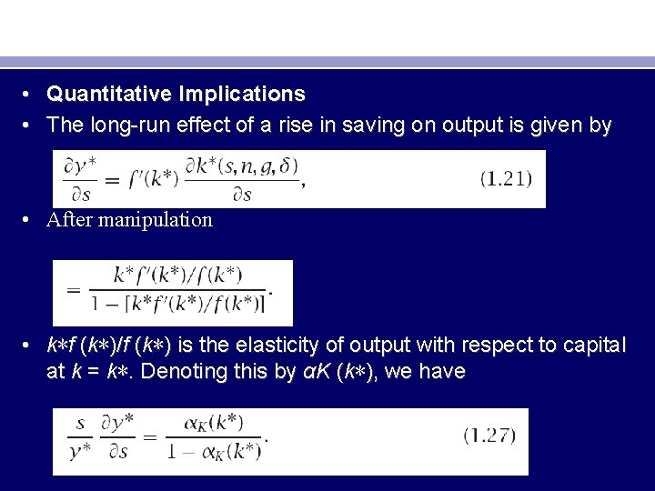
• Quantitative Implications • The long-run effect of a rise in saving on output is given by • After manipulation • k∗f (k∗)/f (k∗) is the elasticity of output with respect to capital at k = k∗. Denoting this by αK (k∗), we have

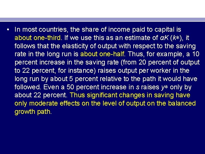
• In most countries, the share of income paid to capital is about one-third. If we use this as an estimate of αK (k∗), it follows that the elasticity of output with respect to the saving rate in the long run is about one-half. Thus, for example, a 10 percent increase in the saving rate (from 20 percent of output to 22 percent, for instance) raises output per worker in the long run by about 5 percent relative to the path it would have followed. Even a 50 percent increase in s raises y∗ only by about 22 percent. Thus significant changes in saving have only moderate effects on the level of output on the balanced growth path.

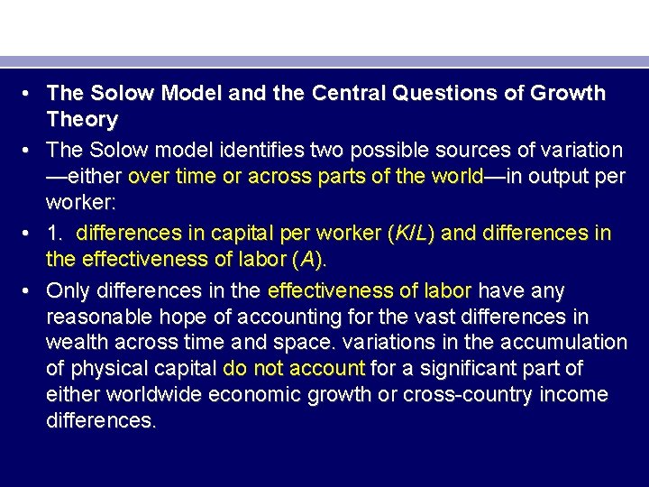
• The Solow Model and the Central Questions of Growth Theory • The Solow model identifies two possible sources of variation —either over time or across parts of the world—in output per worker: • 1. differences in capital per worker (K/L) and differences in the effectiveness of labor (A). • Only differences in the effectiveness of labor have any reasonable hope of accounting for the vast differences in wealth across time and space. variations in the accumulation of physical capital do not account for a significant part of either worldwide economic growth or cross-country income differences.

• Thus differences in K/L cannot account for the differences in output per worker that we observe. • 2. The other potential source of variation in output per worker is the effectiveness of labor. • Unfortunately, however, the Solow model has little to say about the effectiveness of labor. Most obviously, the growth of the effectiveness of labor is exogenous: the model takes as given the behavior of the variable that it identifies as the driving force of growth. • What determines the stock of knowledge over time? • There are other possible interpretations of A: the education and skills of the labor force, the strength of property rights, the quality of infrastructure, cultural attitudes toward entrepreneurship and work, and so on

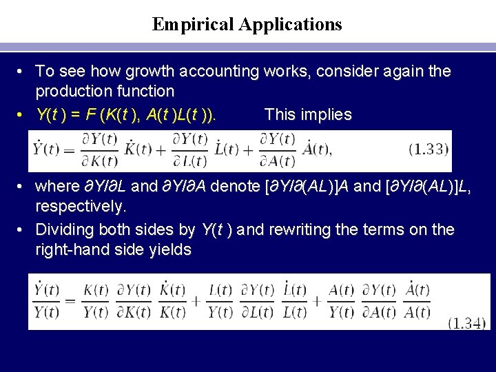
Empirical Applications • To see how growth accounting works, consider again the production function • Y(t ) = F (K(t ), A(t )L(t )). This implies • where ∂Y/∂L and ∂Y/∂A denote [∂Y/∂(AL)]A and [∂Y/∂(AL)]L, respectively. • Dividing both sides by Y(t ) and rewriting the terms on the right-hand side yields

• Here αL(t ) is the elasticity of output with respect to labor at time t, αK (t ) is again the elasticity of output with respect to capital, and R(t ) ≡ [A(t )/Y(t )][∂Y(t )/∂A(t )][ ˙ A(t )/A(t )]. Subtracting ˙L (t )/L(t ) from both sides and using the fact that αL(t ) + αK (t ) = 1 gives an expression for the growth rate of output per worker:

• Thus (1. 35) provides a way of decomposing the growth of output per worker into the contribution of growth of capital per worker and a remaining term, the Solow residual. • The Solow residual is sometimes interpreted as a measure of the contribution of technological progress. • Growth accounting only examines the immediate determinants of growth: it asks how much factor accumulation, improvements in the quality of inputs, and so on contribute to growth while ignoring the deeper issue of what causes the changes in those determinants.

• Growth accounting has been applied to many issues. For example, it has played a major role in a recent debate concerning the exceptionally rapid growth of the newly industrializing countries of East Asia. Young (1995) uses detailed growth accounting to argue that the higher growth in these countries than in the rest of the world is almost entirely due to rising investment, increasing labor force participation, and improving labor quality (in terms of education), and not to rapid technological progress and other forces affecting the Solow residual. • This suggests that for other countries to replicate the NICs’ successes, it is enough for them to promote accumulation of physical and human capital and greater use of resources, and that they need not tackle the even more difficult task of finding ways of obtaining greater output for a given set of inputs.

• Hsieh (2002), however, observes that one can do growth accounting by examining the behavior of factor returns rather than quantities. If rapid growth comes solely from capital accumulation, for example, we will see either a large fall in the return to capital or a large rise in capital’s share (or a combination). Doing the growth accounting this way, Hsieh finds a much larger role for the residual. Young (1998) and Fernald and Neiman (2008) extend the analysis further, and identify reasons that Hsieh’s analysis may have underestimated the role of factor accumulation.

• Growth-accounting studies of the rebound suggest that computers and other types of information technology are the main source of the rebound (see, for example, Oliner and Sichel, 2002, and Oliner, Sichel, and Stiroh, 2007). Until the mid-1990 s, the rapid technological progress in computers and their introduction in many sectors of the economy appear to have had little impact on aggregate productivity In part, this was simply because computers, although spreading rapidly, were still only a small fraction of the overall capital stock.

• Convergence • An issue that has attracted considerable attention in empirical work on growth is whether poor countries tend to grow faster than rich countries. • First, the Solow model predicts that countries converge to their balanced growth paths. Thus to the extent that differences in output per worker arise from countries being at different points relative to their balanced growth paths, one would expect poor countries to catch up to rich ones. • Second, the Solow model implies that the rate of return on capital is lower in countries with more capital per worker. Thus there are incentives for capital to flow from rich to poor countries; this will also tend to cause convergence. • Third, if there are lags in the diffusion of knowledge, income differences can arise because some countries are not yet employing the best available technologies. These differences might tend to shrink as poorer countries gain access to state-of-the-art methods.

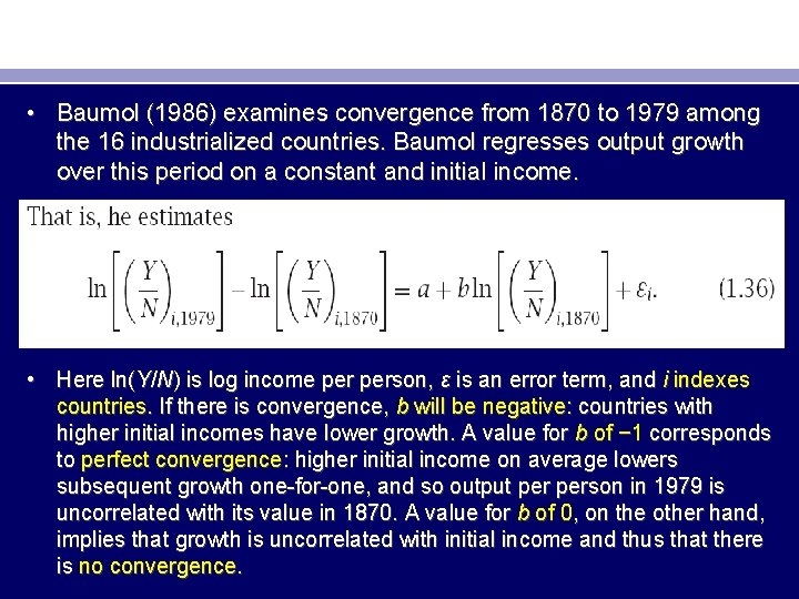
• Baumol (1986) examines convergence from 1870 to 1979 among the 16 industrialized countries. Baumol regresses output growth over this period on a constant and initial income. • Here ln(Y/N) is log income person, ε is an error term, and i indexes countries. If there is convergence, b will be negative: countries with higher initial incomes have lower growth. A value for b of − 1 corresponds to perfect convergence: higher initial income on average lowers subsequent growth one-for-one, and so output person in 1979 is uncorrelated with its value in 1870. A value for b of 0, on the other hand, implies that growth is uncorrelated with initial income and thus that there is no convergence.

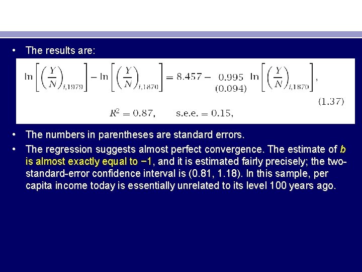
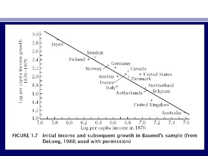
• The results are: • The numbers in parentheses are standard errors. • The regression suggests almost perfect convergence. The estimate of b is almost exactly equal to − 1, and it is estimated fairly precisely; the twostandard-error confidence interval is (0. 81, 1. 18). In this sample, per capita income today is essentially unrelated to its level 100 years ago.

• De. Long (1988) demonstrates, however, that Baumol’s finding is largely spurious. There are two problems. • The first is sample selection. Since historical data are constructed retrospectively, the countries that have long data series are generally those that are the most industrialized today. Thus countries that were not rich 100 years ago are typically in the sample only if they grew rapidly over the next 100 years. Countries that were rich 100 years ago, in contrast, are generally included even if their subsequent growth was only moderate. Because of this, we are likely to see poorer countries growing faster than richer ones in the sample of countries we consider, even if there is no tendency for this to occur on average.

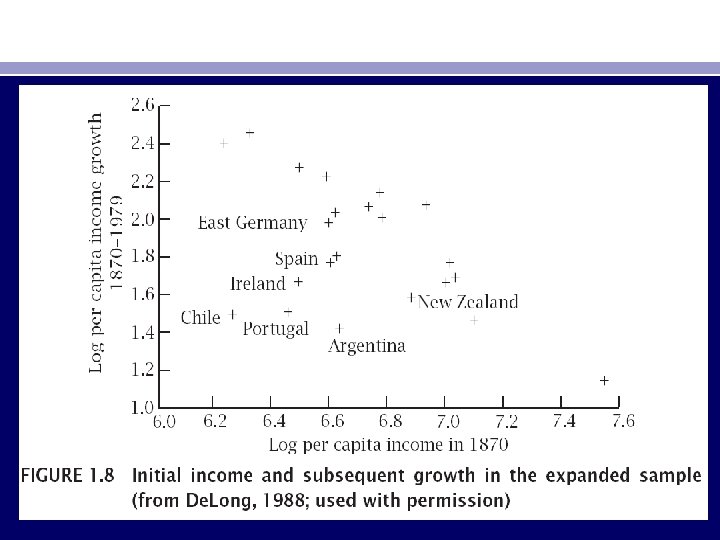
• De. Long therefore considers the richest countries as of 1870; specifically, his sample consists of all countries at least as rich as the second poorest country in Baumol’s sample in 1870, Finland. This causes him to add seven countries to Baumol’s list (Argentina, Chile, East Germany, Ireland, New Zealand, Portugal, and Spain) and to drop one (Japan). 22 • Figure 1. 8 shows the scatterplot for the unbiased sample. The inclusion of the new countries weakens the case for convergence considerably. The regression now produces an estimate of b of − 0. 566, with a standard error of 0. 144. Thus accounting for the selection bias in Baumol’s procedure eliminates about half of the convergence that he finds.

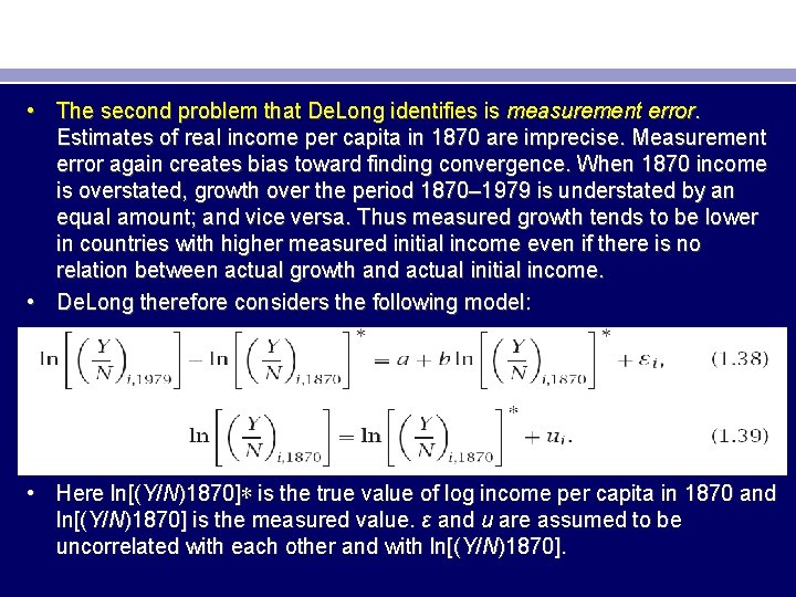
• The second problem that De. Long identifies is measurement error. Estimates of real income per capita in 1870 are imprecise. Measurement error again creates bias toward finding convergence. When 1870 income is overstated, growth over the period 1870– 1979 is understated by an equal amount; and vice versa. Thus measured growth tends to be lower in countries with higher measured initial income even if there is no relation between actual growth and actual initial income. • De. Long therefore considers the following model: • Here ln[(Y/N)1870]∗ is the true value of log income per capita in 1870 and ln[(Y/N)1870] is the measured value. ε and u are assumed to be uncorrelated with each other and with ln[(Y/N)1870].

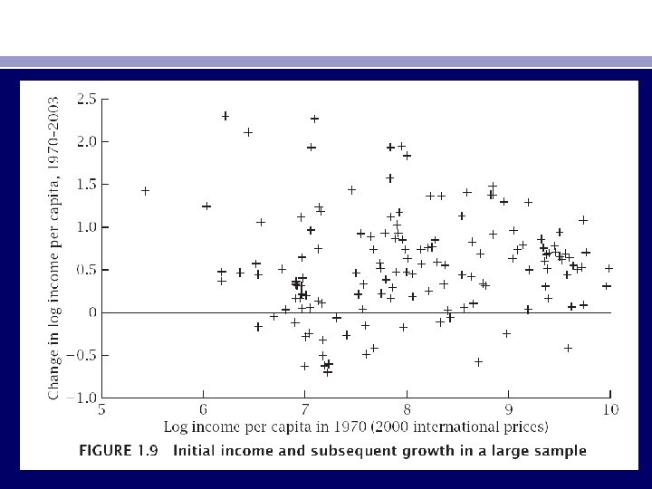
• Figure 1. 9 is a convergence scatterplot analogous to Figures 1. 7 and 1. 8 for virtually the entire non-Communist world for the period 1970– 2003. As the figure shows, there is little evidence of convergence.

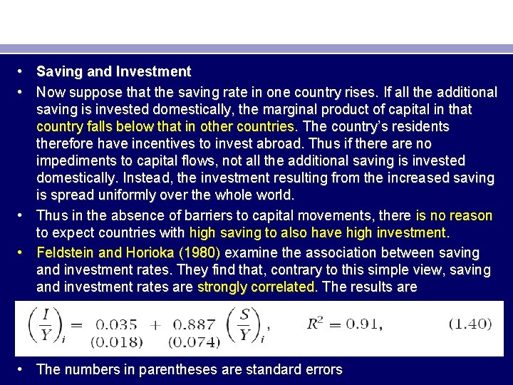
• Saving and Investment • Now suppose that the saving rate in one country rises. If all the additional saving is invested domestically, the marginal product of capital in that country falls below that in other countries. The country’s residents therefore have incentives to invest abroad. Thus if there are no impediments to capital flows, not all the additional saving is invested domestically. Instead, the investment resulting from the increased saving is spread uniformly over the whole world. • Thus in the absence of barriers to capital movements, there is no reason to expect countries with high saving to also have high investment. • Feldstein and Horioka (1980) examine the association between saving and investment rates. They find that, contrary to this simple view, saving and investment rates are strongly correlated. The results are • The numbers in parentheses are standard errors

• Thus, rather than there being no relation between saving and investment, there is an almost one-to-one relation. • Explanations: • One possibility, suggested by Feldstein and Horioka, is that there are significant barriers to capital mobility. In this case, differences in saving and investment across countries would be associated with rate-of-return differences. There is little evidence of such rate-of-return differences, however. • Another possibility is that there are underlying variables that affect both saving and investment. For example, high tax rates can reduce both saving and investment (Barro, Mankiw, and Sala-i-Martin, 1995). Similarly, countries whose citizens have low discount rates, and thus high saving rates, may provide favorable investment climates in ways other than the high saving; for example, they may limit workers’ ability to form strong unions or adopt low tax rates on capital income.

• Finally, the strong association between saving and investment can arise from government policies that offset forces that would otherwise make saving and investment differ. Governments may be averse to large gaps between saving and investment—after all, a large gap must be associated with a large trade deficit (if investment exceeds saving) or a large trade surplus (if saving exceeds investment). If economic forces would otherwise give rise to a large imbalance between saving and investment, the government may choose to adjust its own saving behavior or its tax treatment of saving or investment to bring them into rough balance.

• Helliwell (1998) finds that the saving investment correlation is much weaker if we look across regions within a country rather than across countries. This is certainly consistent with the hypothesis that national governments take steps to prevent large imbalances between aggregate saving and investment, but that such imbalances can develop in the absence of government intervention.