3 1 Vector Quantization VQ Concept Encoding and

3. 1 Vector Quantization (VQ) Concept Encoding and Decoding 3 - 2

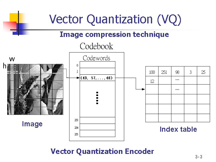
Vector Quantization (VQ) Image compression technique h w Image Index table Vector Quantization Encoder 3 - 3

Vector Quantization (VQ) Image compression technique h w Image Index table Vector Quantization Decoder 3 - 4

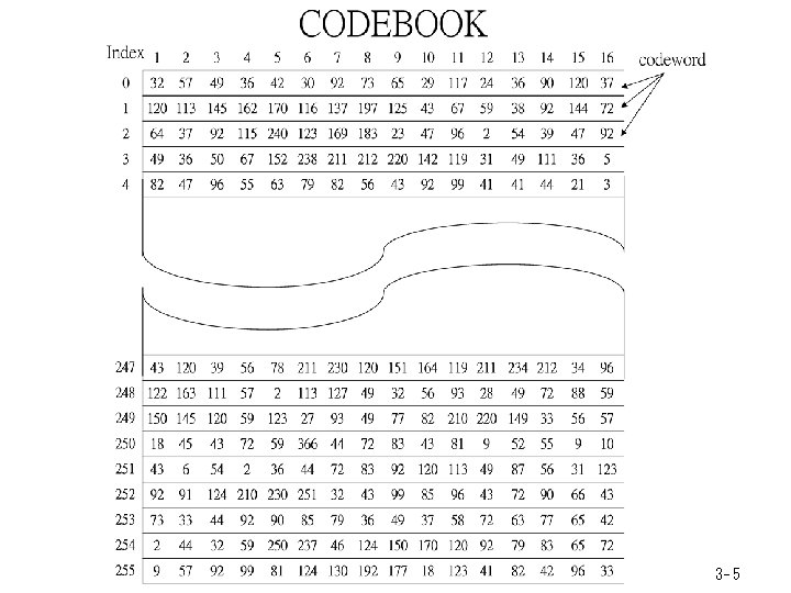
3 - 5

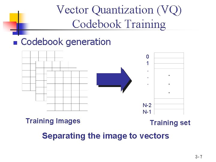
Vector Quantization (VQ) Codebook Training n Codebook generation 0 1. . . N-2 N-1 Training Images Training set Separating the image to vectors 3 - 7

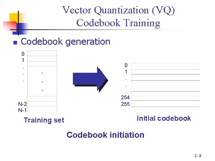
Vector Quantization (VQ) Codebook Training n Codebook generation 0 1. . . N-2 N-1 Training set 0 1. . . 254 255 Initial codebook Codebook initiation 3 - 8

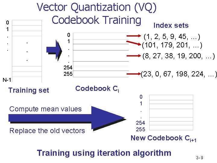
Vector Quantization (VQ) Codebook Training Index sets 0 1. . . 254 255 N-1 Training set (1, 2, 5, 9, 45, …) (101, 179, 201, …) (8, 27, 38, 19, 200, …) (23, 0, 67, 198, 224, …) Codebook Ci Compute mean values Replace the old vectors 0 1. . 254. 255 New Codebook Ci+1 Training using iteration algorithm 3 - 9

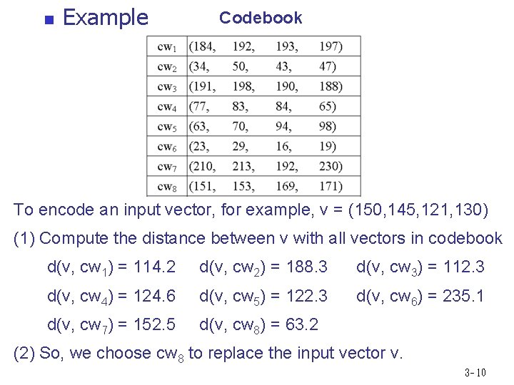
n Example Codebook To encode an input vector, for example, v = (150, 145, 121, 130) (1) Compute the distance between v with all vectors in codebook d(v, cw 1) = 114. 2 d(v, cw 2) = 188. 3 d(v, cw 3) = 112. 3 d(v, cw 4) = 124. 6 d(v, cw 5) = 122. 3 d(v, cw 6) = 235. 1 d(v, cw 7) = 152. 5 d(v, cw 8) = 63. 2 (2) So, we choose cw 8 to replace the input vector v. 3 - 10

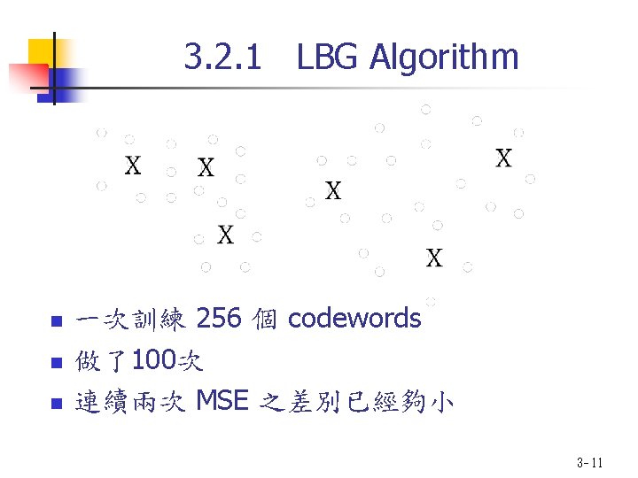
3. 2. 1 LBG Algorithm n n n 一次訓練 256 個 codewords 做了100次 連續兩次 MSE 之差別已經夠小 3 - 11

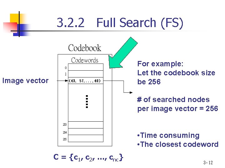
3. 2. 2 Full Search (FS) For example: Let the codebook size be 256 Image vector # of searched nodes per image vector = 256 • Time consuming • The closest codeword C = {c 1, c 2, …, cnc} 3 - 12

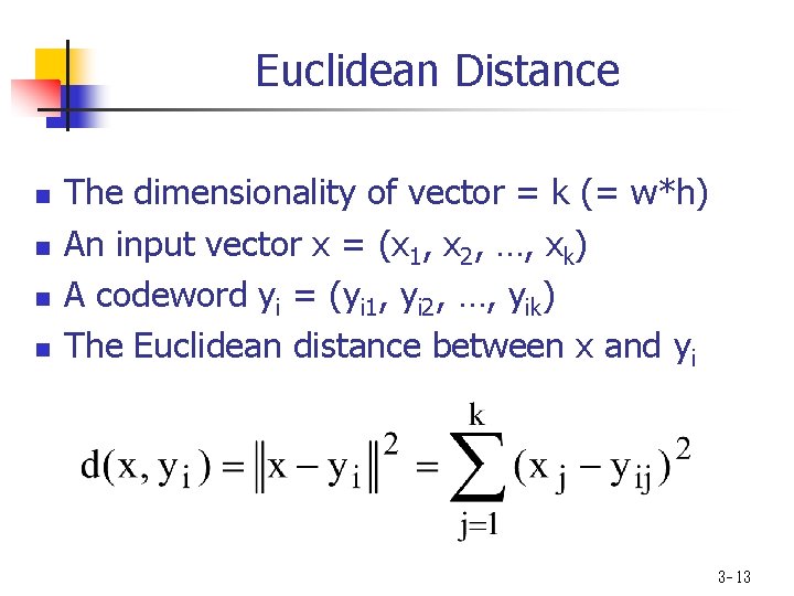
Euclidean Distance n n The dimensionality of vector = k (= w*h) An input vector x = (x 1, x 2, …, xk) A codeword yi = (yi 1, yi 2, …, yik) The Euclidean distance between x and yi 3 - 13

Problem of FS n VQ encoding process (i. e. , codebook search) is time-consuming. n How to speed up the VQ encoder (i. e. , codebook search) is thus an important problem. 3 - 14

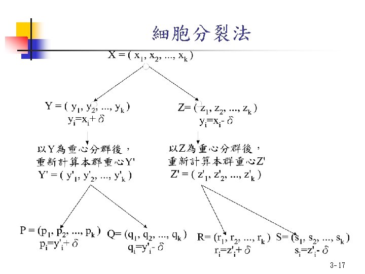
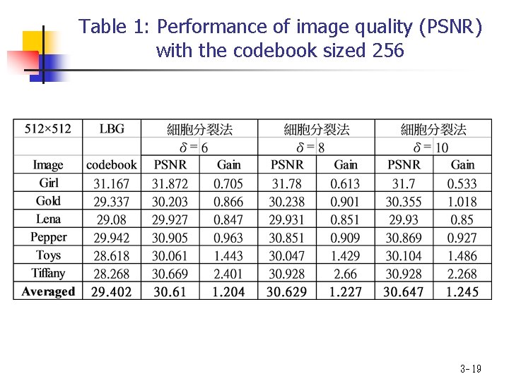
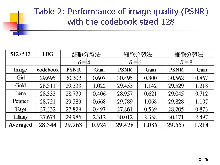
3. 3. 1 細胞分裂法 n Motivation n The distribution of the codewords in the codebook has great influence on the codebook performance. n The codebook initialization is an important part of the VQ codebook design process. n Solve the codebook initialization problem using a tree-structured codebook design process. 3 - 16

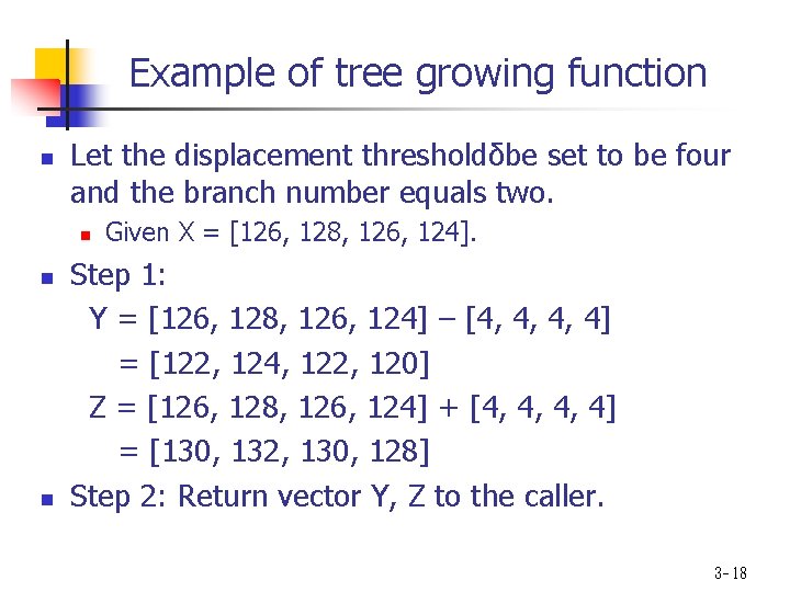
Example of tree growing function n Let the displacement thresholdδbe set to be four and the branch number equals two. n n n Given X = [126, 128, 126, 124]. Step 1: Y = [126, 128, 126, 124] – [4, 4, 4, 4] = [122, 124, 122, 120] Z = [126, 128, 126, 124] + [4, 4, 4, 4] = [130, 132, 130, 128] Step 2: Return vector Y, Z to the caller. 3 - 18

Table 1: Performance of image quality (PSNR) with the codebook sized 256 3 - 19

Table 2: Performance of image quality (PSNR) with the codebook sized 128 3 - 20

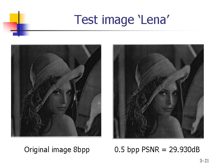
Test image ‘Lena’ Original image 8 bpp 0. 5 bpp PSNR = 29. 930 d. B 3 - 21

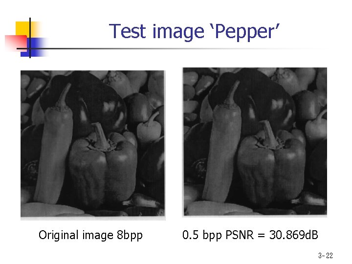
Test image ‘Pepper’ Original image 8 bpp 0. 5 bpp PSNR = 30. 869 d. B 3 - 22

3. 3. 2 結論 n n n Progressively design the codebook using a tree structure. Develop a simple tree growing procedure to generate initial codewords in the training process. Provide better codebook performance than that of the LBG algorithm. 3 - 23

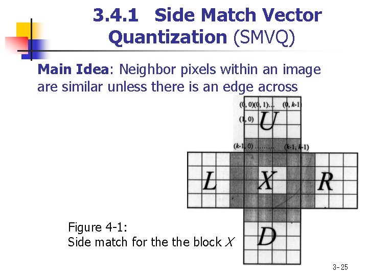
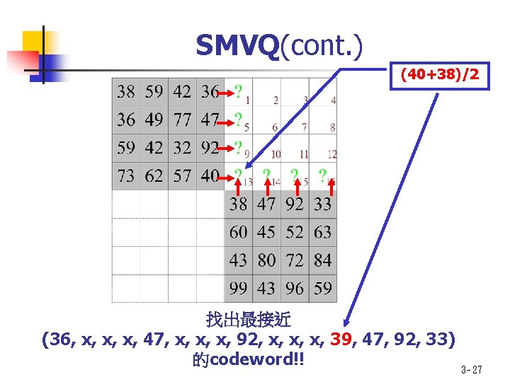
3. 4. 1 Side Match Vector Quantization (SMVQ) Main Idea: Neighbor pixels within an image are similar unless there is an edge across Figure 4 -1: Side match for the block X 3 - 25

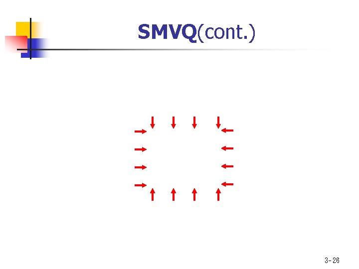
SMVQ(cont. ) 3 - 26

SMVQ(cont. ) (40+38)/2 找出最接近 (36, x, x, x, 47, x, x, x, 92, x, x, x, 39, 47, 92, 33) 的codeword!! 3 - 27

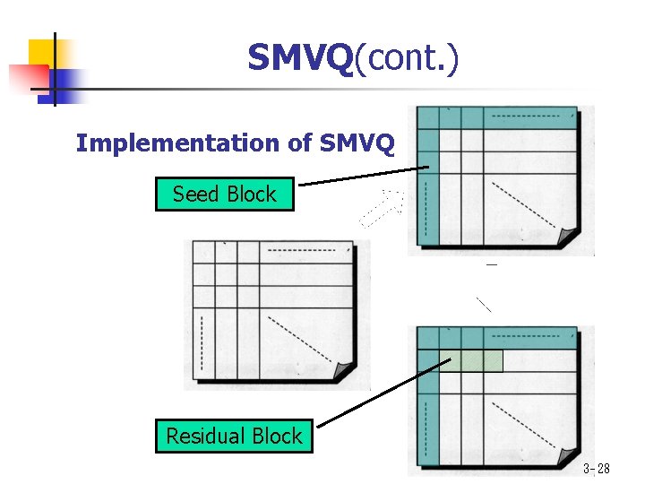
SMVQ(cont. ) Implementation of SMVQ Seed Block Residual Block 3 - 28

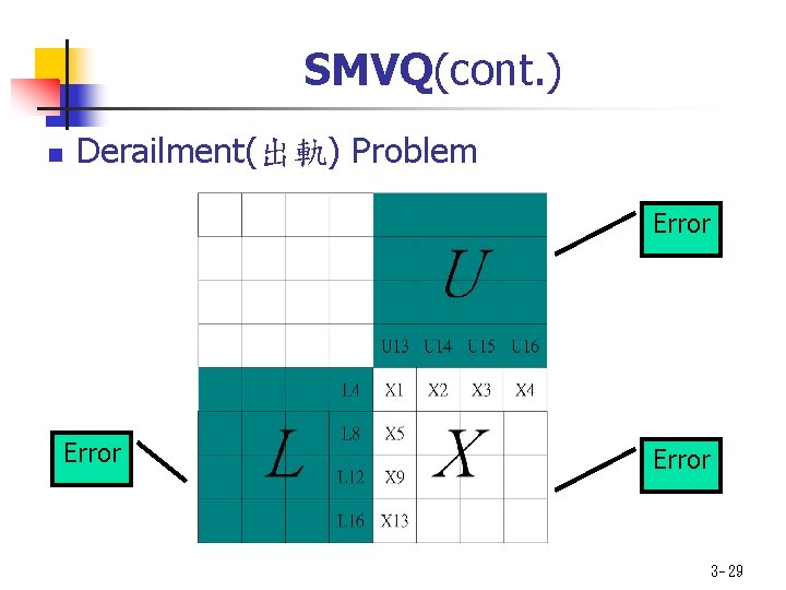
SMVQ(cont. ) n Derailment(出軌) Problem Error 3 - 29

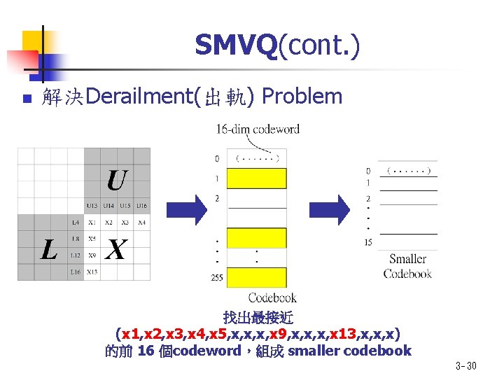
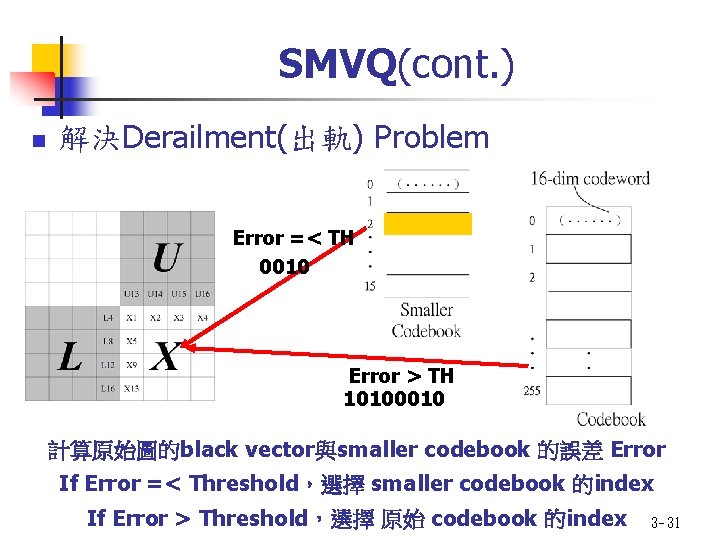
SMVQ(cont. ) n 解決Derailment(出軌) Problem 找出最接近 (x 1, x 2, x 3, x 4, x 5, x, x 9, x, x 13, x, x, x) 的前 16 個codeword，組成 smaller codebook 3 - 30

SMVQ(cont. ) n 解決Derailment(出軌) Problem Error =< TH 0010 Error > TH 10100010 計算原始圖的black vector與smaller codebook 的誤差 Error If Error =< Threshold，選擇 smaller codebook 的index If Error > Threshold，選擇 原始 codebook 的index 3 - 31

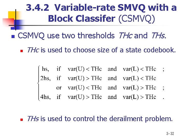
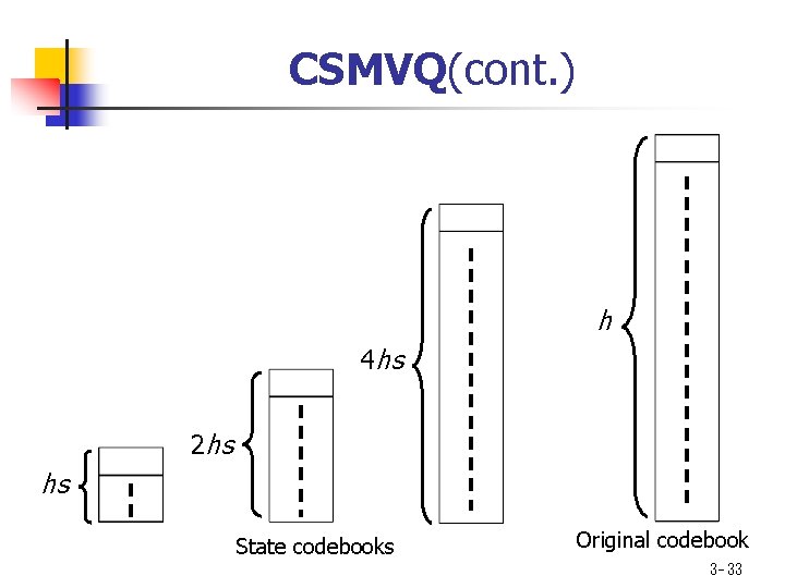
3. 4. 2 Variable-rate SMVQ with a Block Classifer (CSMVQ) n CSMVQ use two thresholds THc and THs. n THc is used to choose size of a state codebook. n THs is used to control the derailment problem. 3 - 32

CSMVQ(cont. ) h 4 hs 2 hs hs State codebooks Original codebook 3 - 33

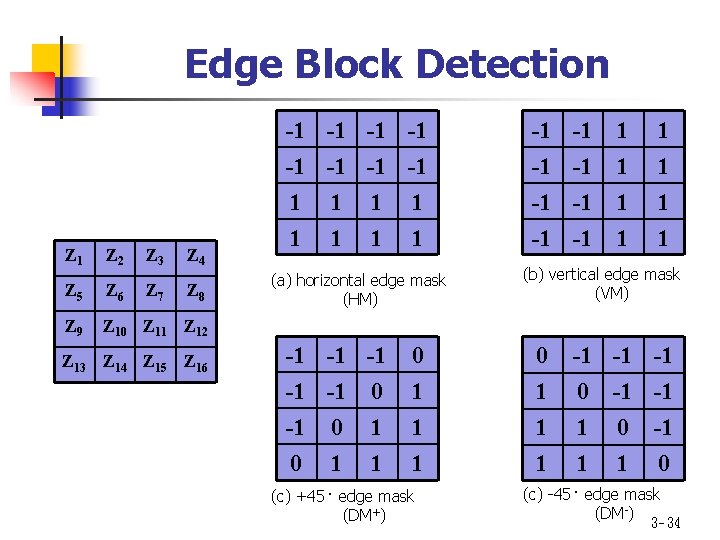
Edge Block Detection Z 1 Z 2 Z 3 Z 7 Z 4 Z 5 Z 6 Z 8 Z 9 Z 10 Z 11 Z 12 Z 13 Z 14 Z 15 Z 16 -1 -1 1 1 1 1 (a) horizontal edge mask (HM) -1 -1 -1 0 1 0 1 1 1 (c) +45。 edge mask (DM+) -1 -1 1 1 1 1 (b) vertical edge mask (VM) 0 1 1 1 -1 -1 -1 0 -1 -1 1 0 -1 1 1 0 (c) -45。 edge mask (DM-) 3 - 34

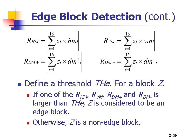
Edge Block Detection (cont. ) n Define a threshold THe. For a block Z. n n If one of the RHM, RVM, RDM+ and RDM- is larger than THe, Z is considered to be an edge block. Otherwise, Z is a non-edge block. 3 - 35

3. 4. 3 Pattern-based SMVQ (PSMVQ) n What is a pattern? n n Why is it called a pattern? n n A pattern is a group of w×w blocks. The encoding order of blocks within a pattern is defined. PSMVQ n n n The Generation of Edge Codebook and Non-edge Codebook The Encoder of PSMVQ The Decoder of PSMVQ 3 - 36

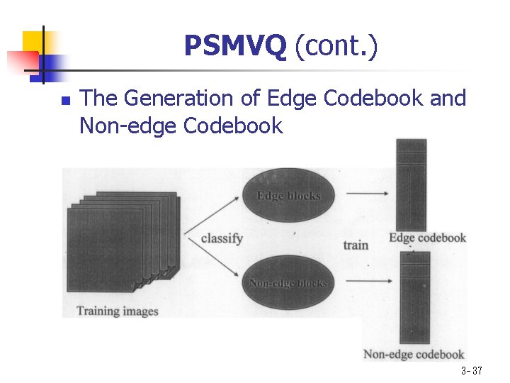
PSMVQ (cont. ) n The Generation of Edge Codebook and Non-edge Codebook 3 - 37

PSMVQ (cont. ) n PSMVQ 1. The map of the block type 2. The definition of the order of seed block generation 3. The adjustment of the order of the seed blocks 4. The encoding order of the residual blocks 3 - 38

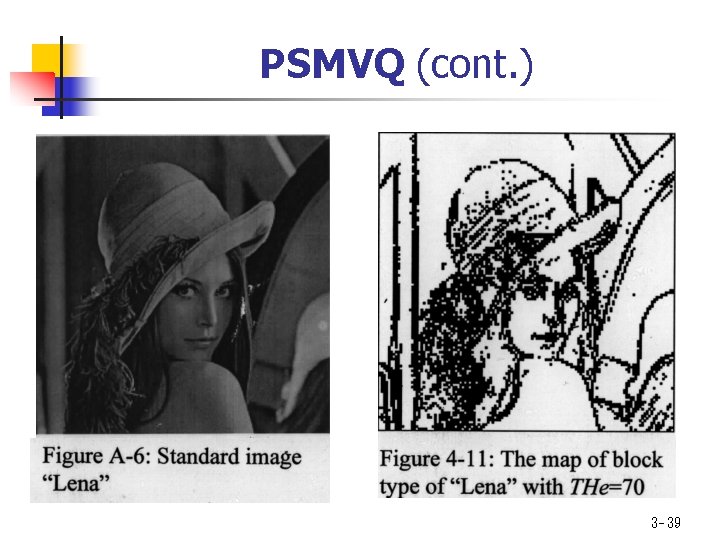
PSMVQ (cont. ) 3 - 39

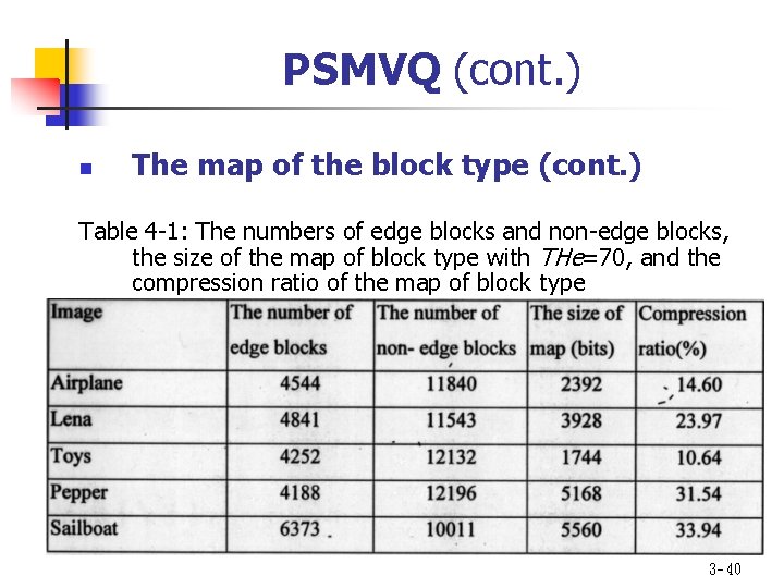
PSMVQ (cont. ) n The map of the block type (cont. ) Table 4 -1: The numbers of edge blocks and non-edge blocks, the size of the map of block type with THe=70, and the compression ratio of the map of block type 3 - 40

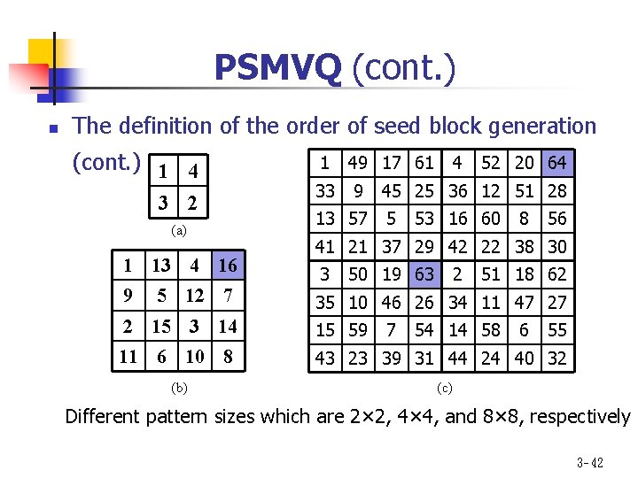
PSMVQ (cont. ) n The definition of the order of seed block generation n Two principles: (1) Uniform (2) The priority of blocks in the right end column and the bottom row will be higher than the other blocks. 3 - 41

PSMVQ (cont. ) n The definition of the order of seed block generation (cont. ) 1 4 3 2 (a) 1 13 4 16 9 5 12 7 1 49 17 61 33 9 13 57 4 52 20 64 45 25 36 12 51 28 5 53 16 60 8 56 41 21 37 29 42 22 38 30 3 50 19 63 2 51 18 62 35 10 46 26 34 11 47 27 2 15 3 14 15 59 11 6 10 8 43 23 39 31 44 24 40 32 (b) (c) 7 54 14 58 6 55 Different pattern sizes which are 2× 2, 4× 4, and 8× 8, respectively 3 - 42

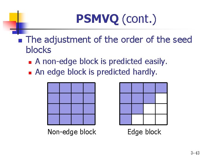
PSMVQ (cont. ) n The adjustment of the order of the seed blocks n n A non-edge block is predicted easily. An edge block is predicted hardly. Non-edge block Edge block 3 - 43

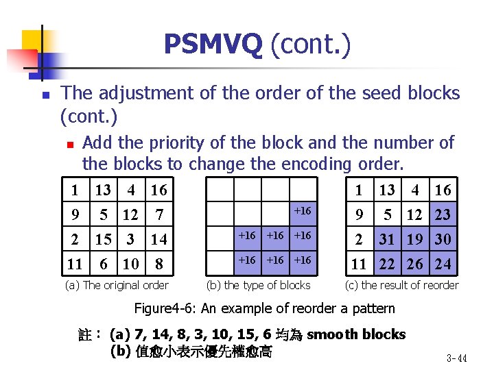
PSMVQ (cont. ) n The adjustment of the order of the seed blocks (cont. ) n Add the priority of the block and the number of the blocks to change the encoding order. 1 13 4 16 9 5 12 7 +16 2 15 3 14 11 6 10 8 +16 +16 (a) The original order (b) the type of blocks +16 +16 1 9 2 11 13 5 31 22 4 12 19 26 16 23 30 24 (c) the result of reorder Figure 4 -6: An example of reorder a pattern 註： (a) 7, 14, 8, 3, 10, 15, 6 均為 smooth blocks (b) 值愈小表示優先權愈高 3 - 44

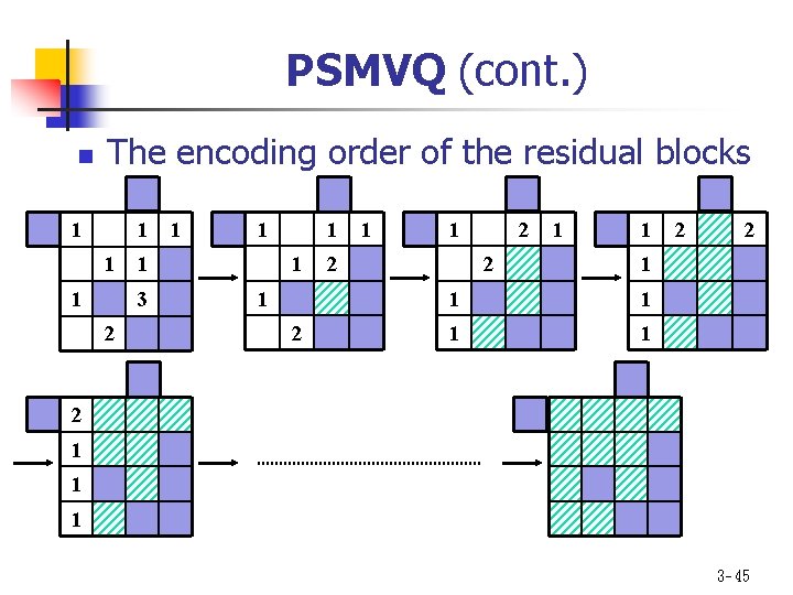
PSMVQ (cont. ) n The encoding order of the residual blocks 1 1 1 1 3 2 1 1 2 2 2 1 1 1 1 1 2 1 1 1 3 - 45

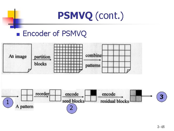
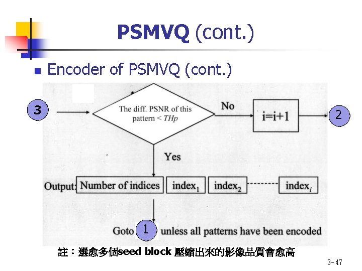
PSMVQ (cont. ) n 1 Encoder of PSMVQ 3 2 3 - 46

PSMVQ (cont. ) n Encoder of PSMVQ (cont. ) 3 2 1 註：選愈多個seed block 壓縮出來的影像品質會愈高 3 - 47

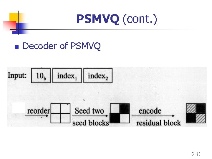
PSMVQ (cont. ) n Decoder of PSMVQ 3 - 48

Experimental results of PSMVQ n Experimental Environment n n n n Linux operation system Pentium 233 Training set: “Airplane”, “Lena”, “Barb”, “Boat”, and “Toys” Testing images: “Airplane”, “Lena”, “Toys”, “Girl” and “Pepper” Images size: 512× 512 pixels Image color: 256 gray levels Block size: 4× 4 pixels 3 - 49

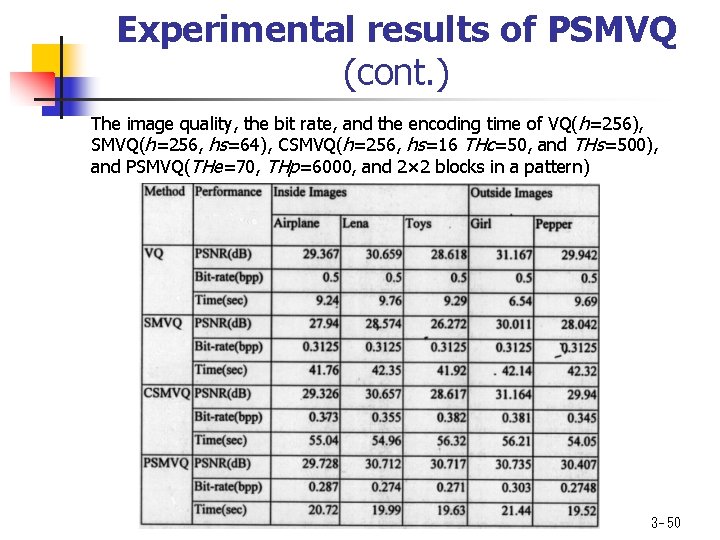
Experimental results of PSMVQ (cont. ) The image quality, the bit rate, and the encoding time of VQ( h=256), SMVQ(h=256, hs=64), CSMVQ(h=256, hs=16 THc=50, and THs=500), and PSMVQ(THe=70, THp=6000, and 2× 2 blocks in a pattern) 3 - 50

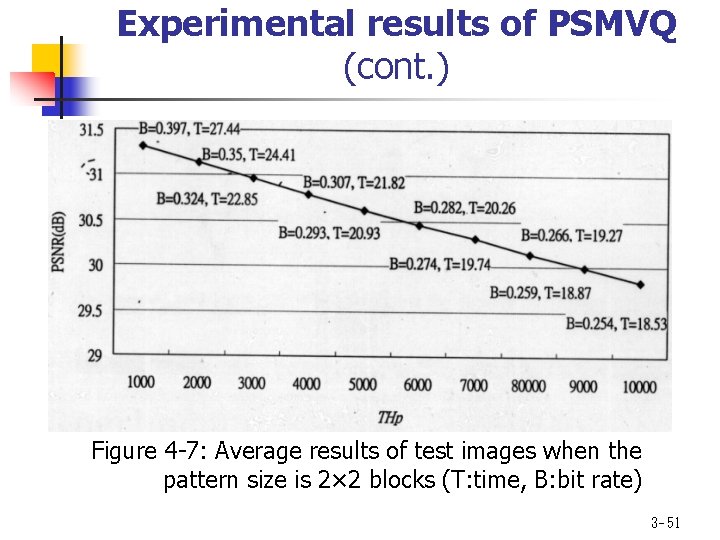
Experimental results of PSMVQ (cont. ) Figure 4 -7: Average results of test images when the pattern size is 2× 2 blocks (T: time, B: bit rate) 3 - 51

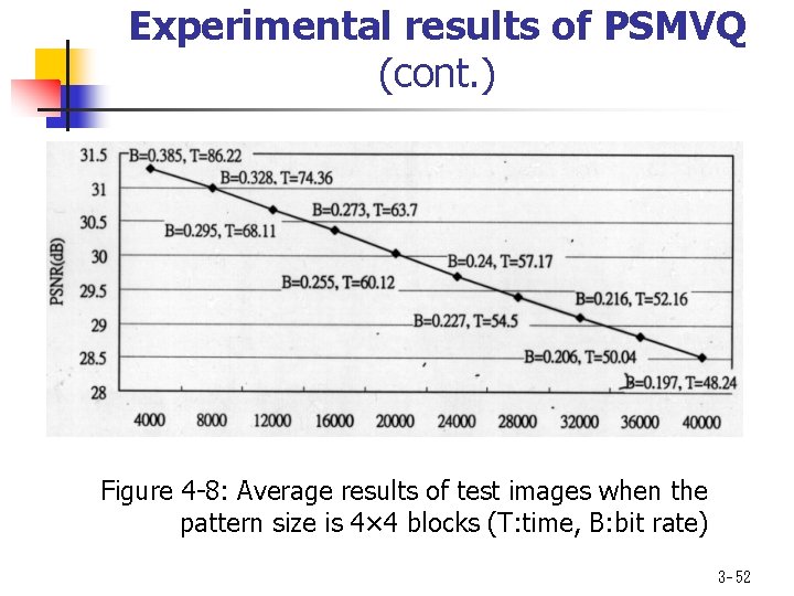
Experimental results of PSMVQ (cont. ) Figure 4 -8: Average results of test images when the pattern size is 4× 4 blocks (T: time, B: bit rate) 3 - 52

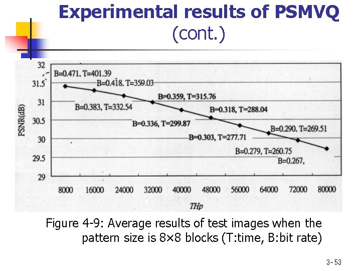
Experimental results of PSMVQ (cont. ) Figure 4 -9: Average results of test images when the pattern size is 8× 8 blocks (T: time, B: bit rate) 3 - 53

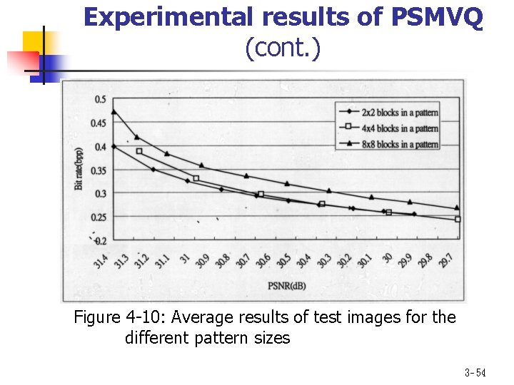
Experimental results of PSMVQ (cont. ) Figure 4 -10: Average results of test images for the different pattern sizes 3 - 54

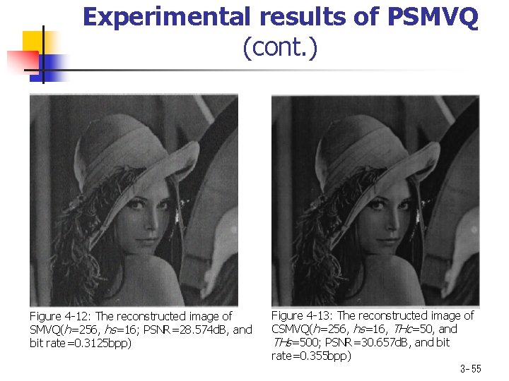
Experimental results of PSMVQ (cont. ) Figure 4 -12: The reconstructed image of SMVQ(h=256, hs=16; PSNR=28. 574 d. B, and bit rate=0. 3125 bpp) Figure 4 -13: The reconstructed image of CSMVQ(h=256, hs=16, THc=50, and THs=500; PSNR=30. 657 d. B, and bit rate=0. 355 bpp) 3 - 55

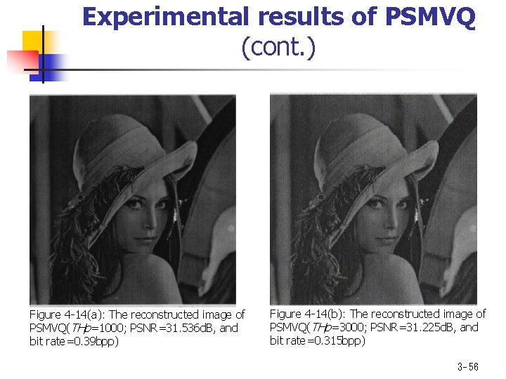
Experimental results of PSMVQ (cont. ) Figure 4 -14(a): The reconstructed image of PSMVQ(THp=1000; PSNR=31. 536 d. B, and bit rate=0. 39 bpp) Figure 4 -14(b): The reconstructed image of PSMVQ(THp=3000; PSNR=31. 225 d. B, and bit rate=0. 315 bpp) 3 - 56

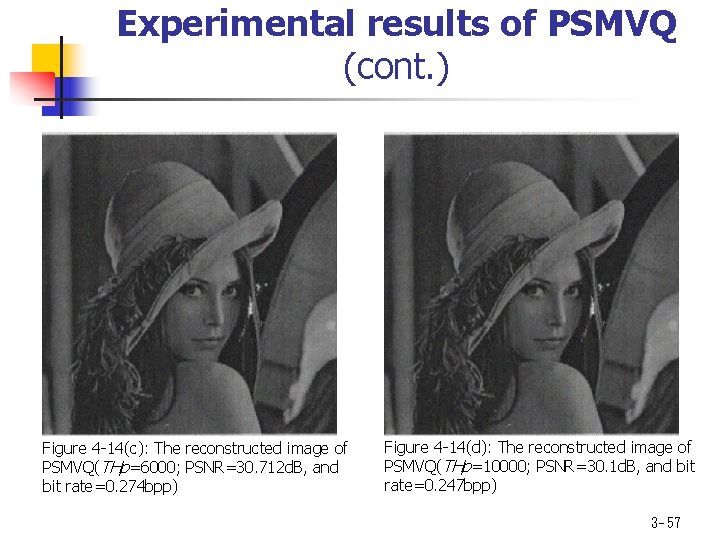
Experimental results of PSMVQ (cont. ) Figure 4 -14(c): The reconstructed image of PSMVQ(THp=6000; PSNR=30. 712 d. B, and bit rate=0. 274 bpp) Figure 4 -14(d): The reconstructed image of PSMVQ(THp=10000; PSNR=30. 1 d. B, and bit rate=0. 247 bpp) 3 - 57