DEPARTMENT OF COMPUTER SCIENCE UNIVERSITY OF JOENSUU FINLAND

DEPARTMENT OF COMPUTER SCIENCE UNIVERSITY OF JOENSUU, FINLAND Image Compression Lecture 9 Optimal Scalar Quantization Alexander Kolesnikov

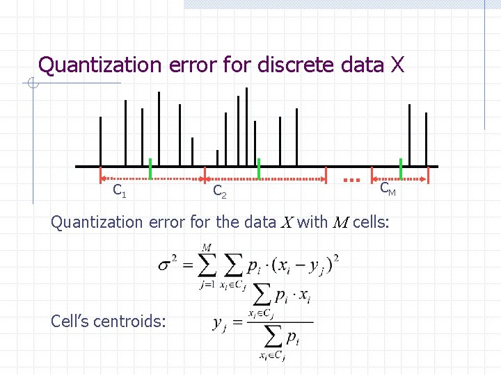
Quantization error for discrete data X C 1 C 2 . . . CM Quantization error for the data X with M cells: Cell’s centroids:

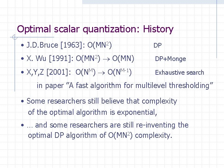
Optimal scalar quantization: History • J. D. Bruce [1963]: O(MN 2) DP • X. Wu [1991]: O(MN 2) O(MN) DP+Monge • X, Y, Z [2001]: O(NM) O(NM-1) Exhaustive search in paper ”A fast algorithm for multilevel thresholding” • Some researchers still believe that complexity of the optimal algorithm is exponential, • … and some researchers are still re-inventing the optimal DP algorithm of O(MN 2) complexity.

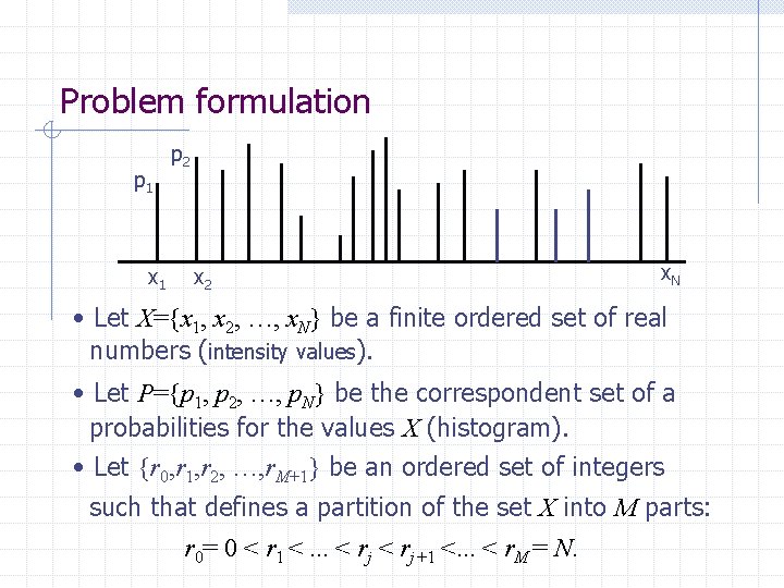
Problem formulation p 1 x 1 p 2 x. N • Let X={x 1, x 2, …, x. N} be a finite ordered set of real numbers (intensity values). • Let P={p 1, p 2, …, p. N} be the correspondent set of a probabilities for the values X (histogram). • Let {r 0, r 1, r 2, …, r. M+1} be an ordered set of integers such that defines a partition of the set X into M parts: r 0= 0 < r 1 <. . . < rj+1 <. . . < r. M = N.

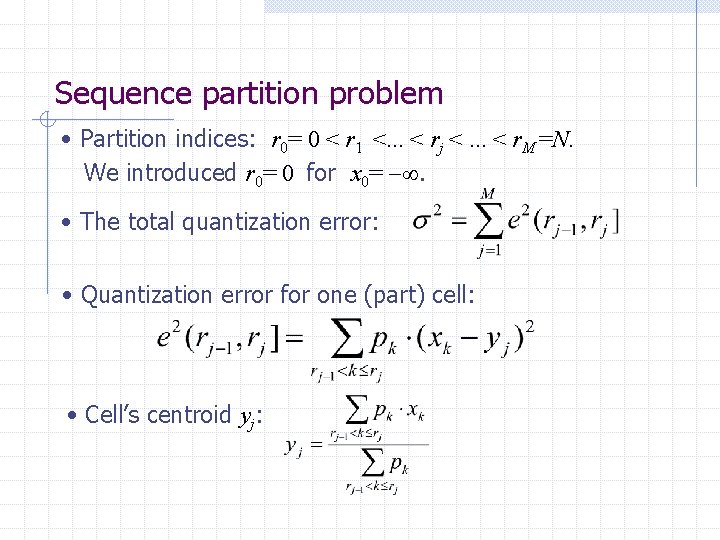
Sequence partition problem • Partition indices: r 0= 0 < r 1 <. . . < rj <. . . < r. M =N. We introduced r 0= 0 for x 0= . • The total quantization error: • Quantization error for one (part) cell: • Cell’s centroid yj:

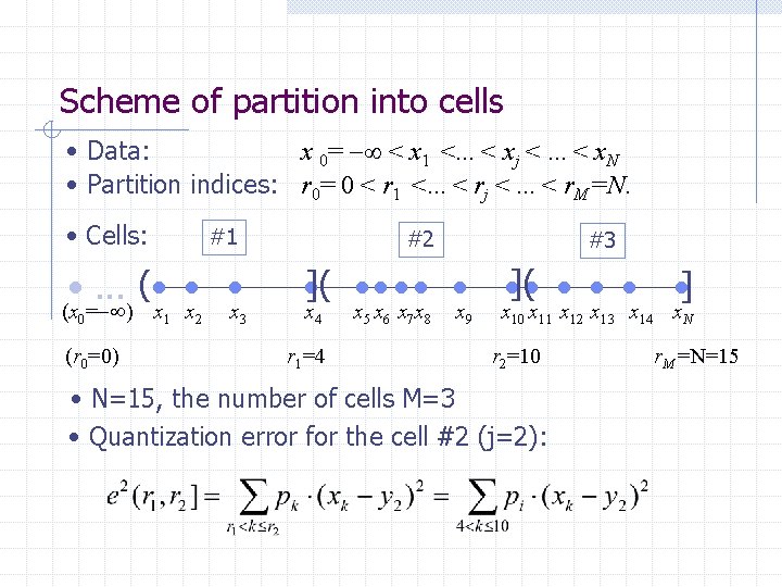
Scheme of partition into cells • Data: x 0= < x 1 <. . . < xj <. . . < x. N • Partition indices: r 0= 0 < r 1 <. . . < rj <. . . < r. M =N. • Cells: #1 • . . . ( • • • (x 0= ) (r 0=0) x 1 x 2 x 3 #2 #3 • ]( • • • x 4 r 1=4 x 5 x 6 x 7 x 8 x 9 • ]( • • • ] x 10 x 11 x 12 x 13 x 14 x. N r 2=10 • N=15, the number of cells M=3 • Quantization error for the cell #2 (j=2): r. M =N=15

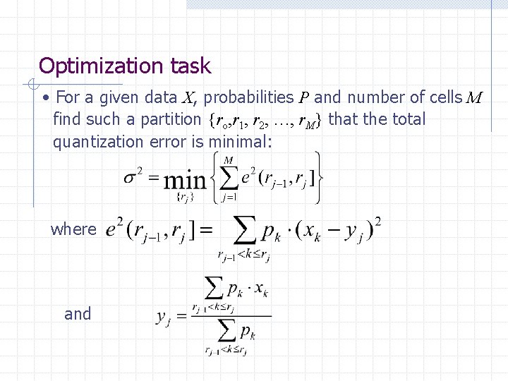
Optimization task • For a given data X, probabilities P and number of cells M find such a partition {ro, r 1, r 2, …, r. M} that the total quantization error is minimal: where and

Cost function DM(0, N] Let us introduce cost function Dm(0, n] that is minimum quantization error for quantization of data sub-set Xn={x 1, x 2, …, xn} with m cells: Then DM(0, N] gives us solution of the problem in question.

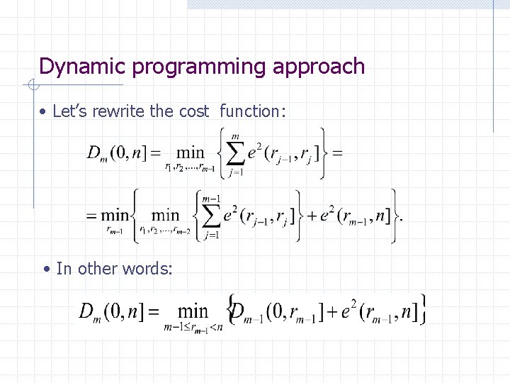
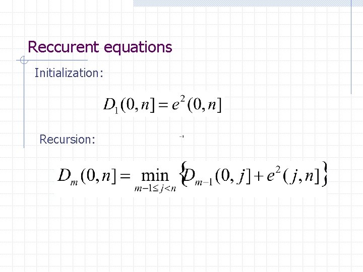
Dynamic programming approach • Let’s rewrite the cost function: • In other words:

Reccurent equations Initialization: Recursion:

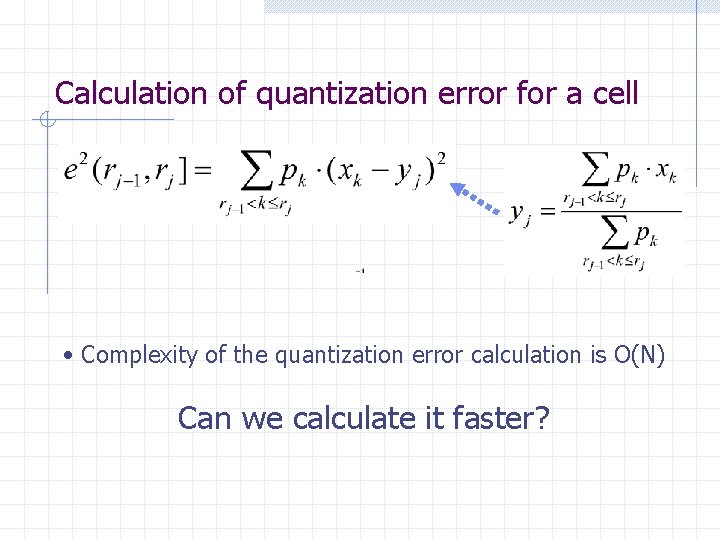
Calculation of quantization error for a cell • Complexity of the quantization error calculation is O(N) Can we calculate it faster?

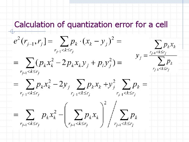
Calculation of quantization error for a cell

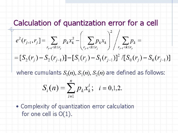
Calculation of quantization error for a cell where cumulants S 0(n), S 1(n), S 2(n) are defined as follows: • Complexity of quantization error calculation for one cell is O(1).

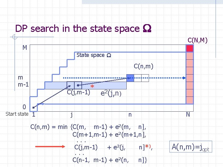
DP search in the state space C(N, M) b M State space C(n, m) m m-1 C(j, m-1) 0 Start state 1 j * e 2(j, n) n C(n, m) = min {C(m, m-1) + e 2(m, n], C(m+1, m-1) + e 2(m+1, n], . . . C(j, m-1) + e 2(j, n]*), . . . C(n-1, m-1) + e 2(n, n]} N A(n, m)=jopt

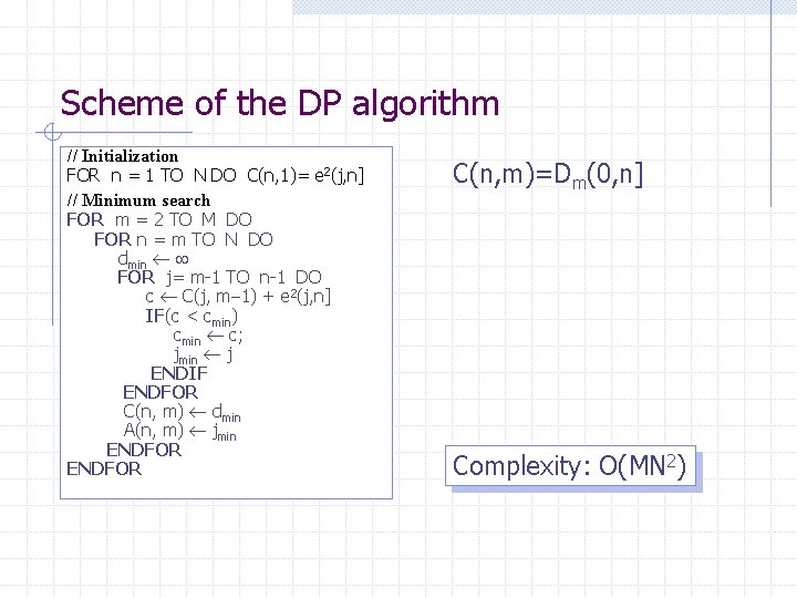
Scheme of the DP algorithm // Initialization FOR n = 1 TO N DO C(n, 1)= e 2(j, n] // Minimum search FOR m = 2 TO M DO FOR n = m TO N DO dmin FOR j= m-1 TO n-1 DO c C(j, m 1) + e 2(j, n] IF(c < cmin) cmin c; jmin j ENDIF ENDFOR C(n, m) dmin A(n, m) jmin ENDFOR C(n, m)=Dm(0, n] Complexity: O(MN 2)

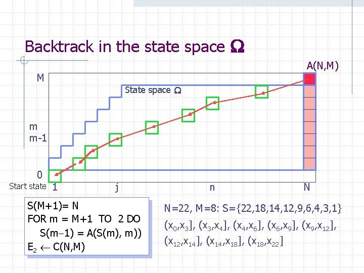
Backtrack in the state space A(N, M) b M State space m m-1 0 Start state 1 j S(M+1)= N FOR m = M+1 TO 2 DO S(m 1) = A(S(m), m)) E 2 C(N, M) n N N=22, M=8: S={22, 18, 14, 12, 9, 6, 4, 3, 1} (x 0, x 3], (x 3, x 4], (x 4, x 6], (x 6, x 9], (x 9, x 12], (x 12, x 14], (x 14, x 18], (x 18, x 22]

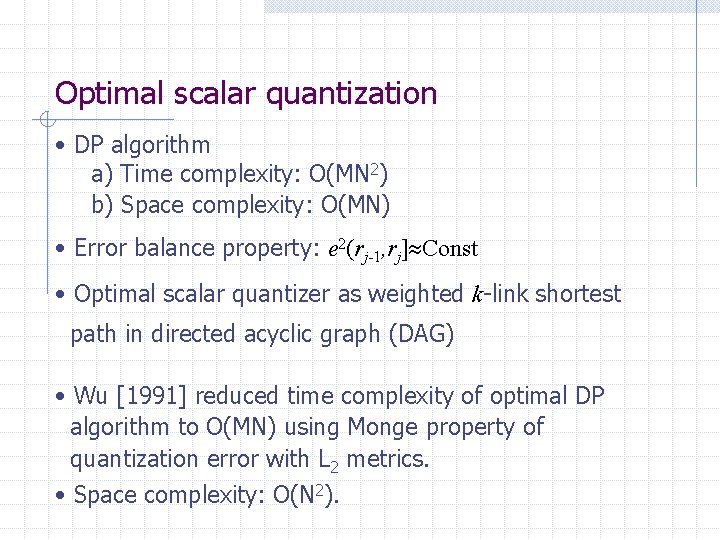
Optimal scalar quantization • DP algorithm a) Time complexity: O(MN 2) b) Space complexity: O(MN) • Error balance property: e 2(rj-1, rj] Const • Optimal scalar quantizer as weighted k-link shortest path in directed acyclic graph (DAG) • Wu [1991] reduced time complexity of optimal DP algorithm to O(MN) using Monge property of quantization error with L 2 metrics. • Space complexity: O(N 2).

Can we do it faster? • Wu [1991] reduced time complexity of optimal DP algorithm to O(MN) using Monge property (monotonicity property) of quantization error with L 2 metrics. • Space complexity: O(N 2).

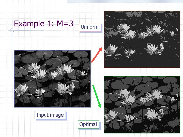
Example 1: M=3 Uniform Input image Optimal

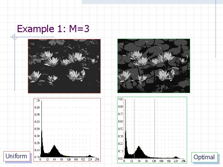
Example 1: M=3 Uniform Optimal

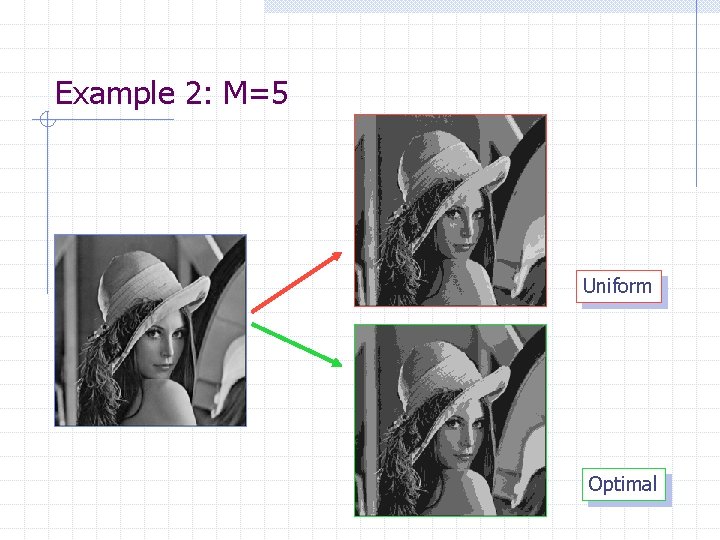
Example 2: M=5 Uniform Optimal

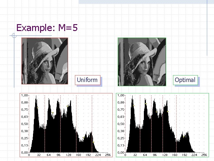
Example: M=5 Uniform Optimal

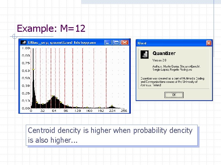
Example: M=12 Centroid dencity is higher when probability dencity is also higher. . .

Summary 1) Optimal scalar quantization