15 Multiple Integrals Copyright Cengage Learning All rights

15 Multiple Integrals Copyright © Cengage Learning. All rights reserved.

15. 5 Applications of Double Integrals Copyright © Cengage Learning. All rights reserved.

Density and Mass 3

Density and Mass We were able to use single integrals to compute moments and the center of mass of a thin plate or lamina with constant density. But now, equipped with the double integral, we can consider a lamina with variable density. Suppose the lamina occupies a region D of the xy-plane and its density (in units of mass per unit area) at a point (x, y) in D is given by (x, y), where is a continuous function on D. 4

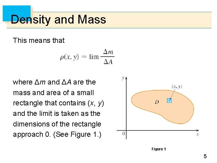
Density and Mass This means that where Δm and ΔA are the mass and area of a small rectangle that contains (x, y) and the limit is taken as the dimensions of the rectangle approach 0. (See Figure 1. ) Figure 1 5

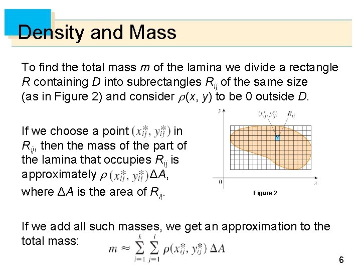
Density and Mass To find the total mass m of the lamina we divide a rectangle R containing D into subrectangles Rij of the same size (as in Figure 2) and consider (x, y) to be 0 outside D. If we choose a point in Rij, then the mass of the part of the lamina that occupies Rij is approximately ΔA, where ΔA is the area of Rij. Figure 2 If we add all such masses, we get an approximation to the total mass: 6

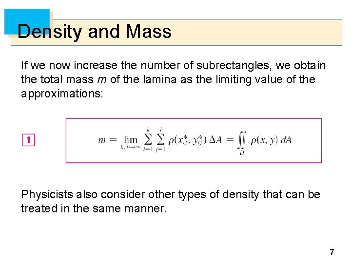
Density and Mass If we now increase the number of subrectangles, we obtain the total mass m of the lamina as the limiting value of the approximations: Physicists also consider other types of density that can be treated in the same manner. 7

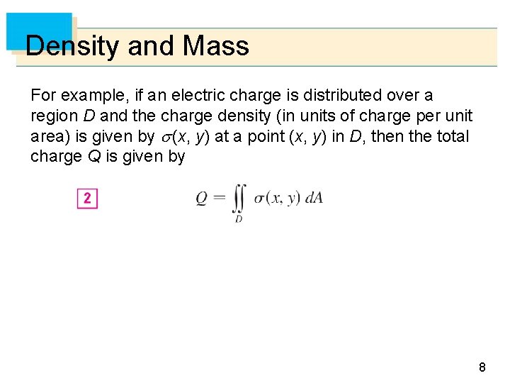
Density and Mass For example, if an electric charge is distributed over a region D and the charge density (in units of charge per unit area) is given by (x, y) at a point (x, y) in D, then the total charge Q is given by 8

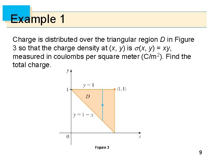
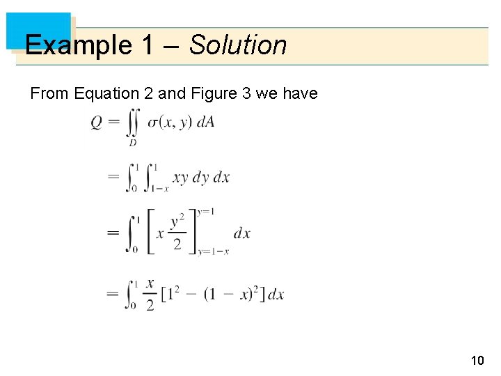
Example 1 Charge is distributed over the triangular region D in Figure 3 so that the charge density at (x, y) is (x, y) = xy, measured in coulombs per square meter (C/m 2). Find the total charge. Figure 3 9

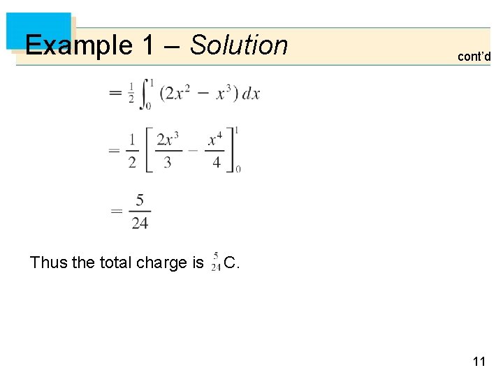
Example 1 – Solution From Equation 2 and Figure 3 we have 10

Example 1 – Solution Thus the total charge is cont’d C. 11

Moments and Centers of Mass 12

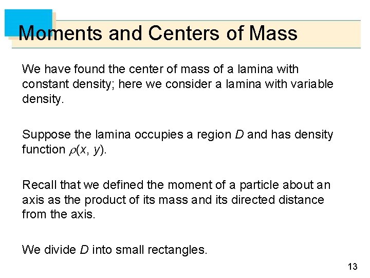
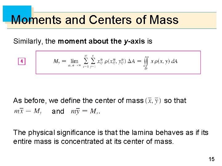
Moments and Centers of Mass We have found the center of mass of a lamina with constant density; here we consider a lamina with variable density. Suppose the lamina occupies a region D and has density function (x, y). Recall that we defined the moment of a particle about an axis as the product of its mass and its directed distance from the axis. We divide D into small rectangles. 13

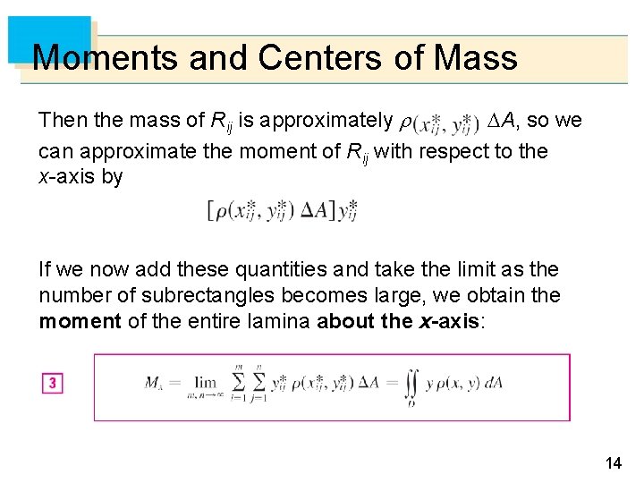
Moments and Centers of Mass Then the mass of Rij is approximately A, so we can approximate the moment of Rij with respect to the x-axis by If we now add these quantities and take the limit as the number of subrectangles becomes large, we obtain the moment of the entire lamina about the x-axis: 14

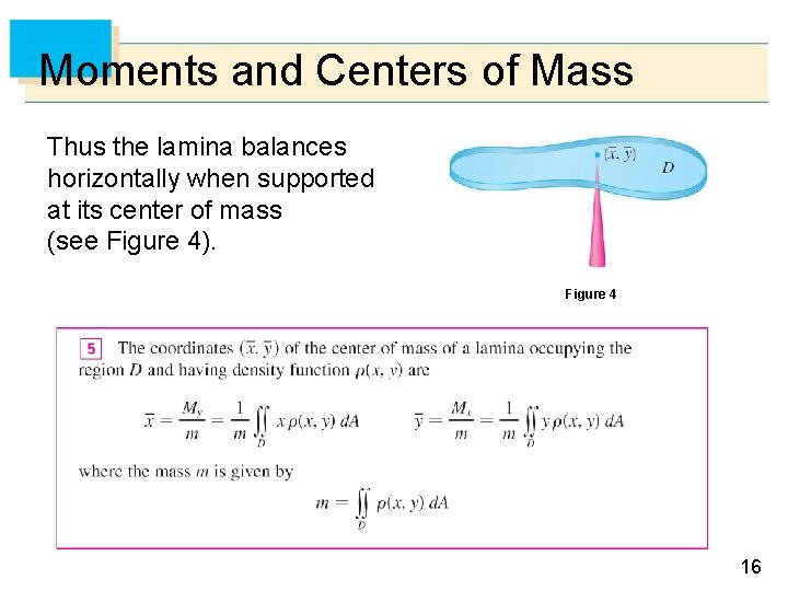
Moments and Centers of Mass Similarly, the moment about the y-axis is As before, we define the center of mass and so that The physical significance is that the lamina behaves as if its entire mass is concentrated at its center of mass. 15

Moments and Centers of Mass Thus the lamina balances horizontally when supported at its center of mass (see Figure 4). Figure 4 16

Moment of Inertia 17

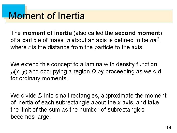
Moment of Inertia The moment of inertia (also called the second moment) of a particle of mass m about an axis is defined to be mr 2, where r is the distance from the particle to the axis. We extend this concept to a lamina with density function (x, y) and occupying a region D by proceeding as we did for ordinary moments. We divide D into small rectangles, approximate the moment of inertia of each subrectangle about the x-axis, and take the limit of the sum as the number of subrectangles becomes large. 18

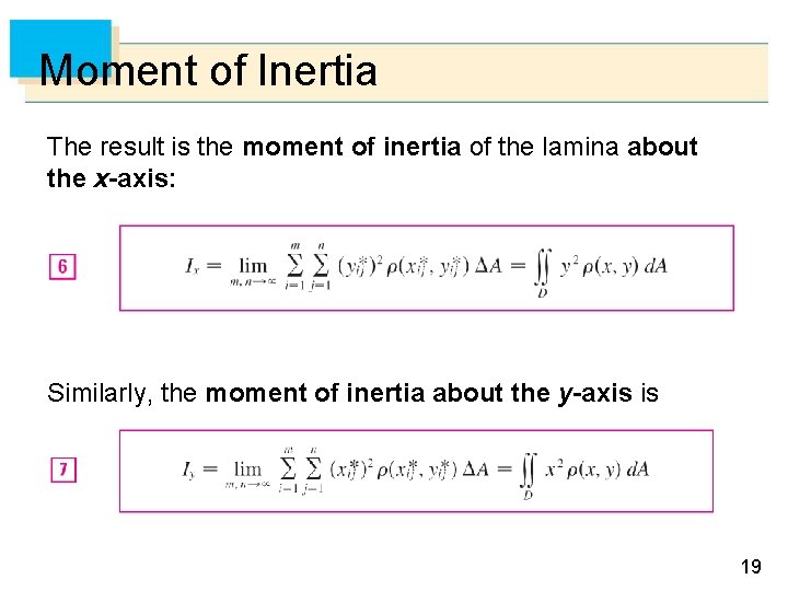
Moment of Inertia The result is the moment of inertia of the lamina about the x-axis: Similarly, the moment of inertia about the y-axis is 19

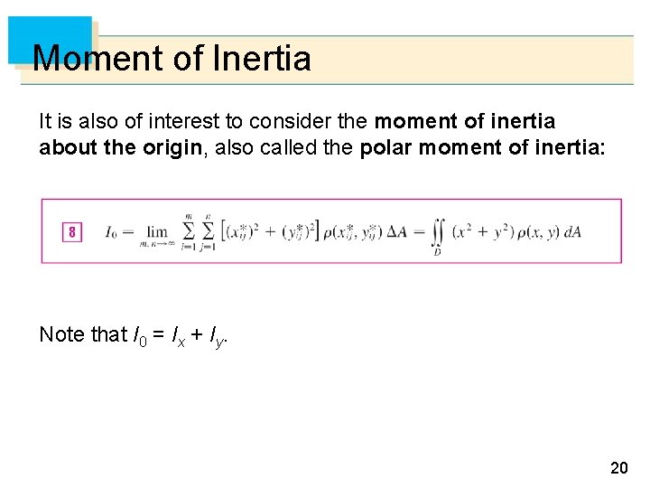
Moment of Inertia It is also of interest to consider the moment of inertia about the origin, also called the polar moment of inertia: Note that I 0 = Ix + Iy. 20

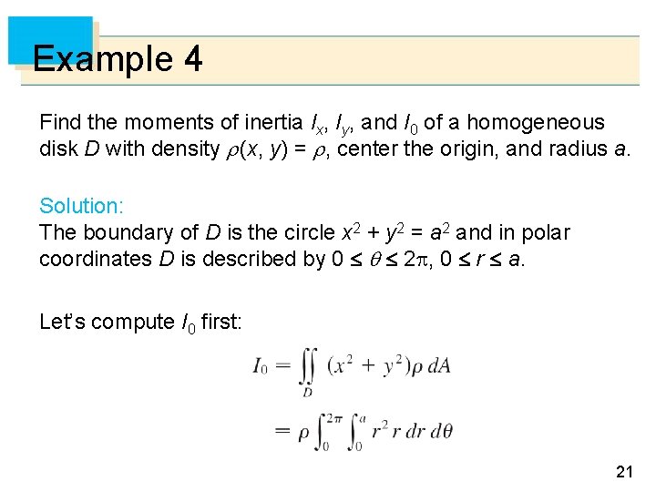
Example 4 Find the moments of inertia Ix, Iy, and I 0 of a homogeneous disk D with density (x, y) = , center the origin, and radius a. Solution: The boundary of D is the circle x 2 + y 2 = a 2 and in polar coordinates D is described by 0 2 , 0 r a. Let’s compute I 0 first: 21

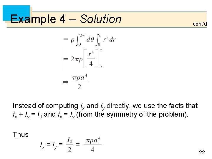
Example 4 – Solution cont’d Instead of computing Ix and Iy directly, we use the facts that Ix + Iy = I 0 and Ix = Iy (from the symmetry of the problem). Thus I x = Iy = = 22

Moment of Inertia In Example 4 notice that the mass of the disk is m = density area = ( a 2) so the moment of inertia of the disk about the origin (like a wheel about its axle) can be written as Thus if we increase the mass or the radius of the disk, we thereby increase the moment of inertia. 23

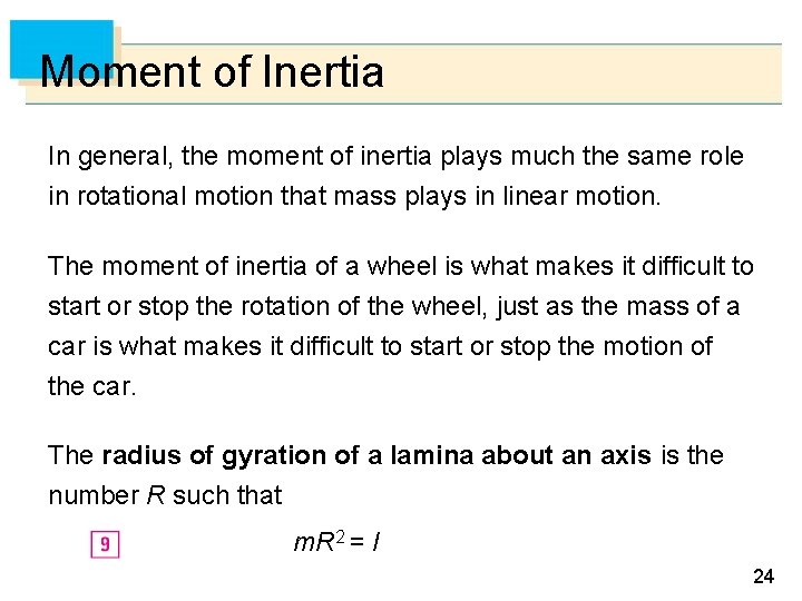
Moment of Inertia In general, the moment of inertia plays much the same role in rotational motion that mass plays in linear motion. The moment of inertia of a wheel is what makes it difficult to start or stop the rotation of the wheel, just as the mass of a car is what makes it difficult to start or stop the motion of the car. The radius of gyration of a lamina about an axis is the number R such that m. R 2 = I 24

Moment of Inertia Where m is the mass of the lamina I and is the moment of inertia about the given axis. Equation 9 says that if the mass of the lamina were concentrated at a distance R from the axis, then the moment of inertia of this “point mass” would be the same as the moment of inertia of the lamina. 25

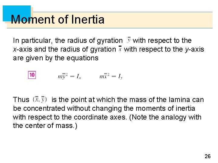
Moment of Inertia In particular, the radius of gyration with respect to the x-axis and the radius of gyration with respect to the y-axis are given by the equations Thus is the point at which the mass of the lamina can be concentrated without changing the moments of inertia with respect to the coordinate axes. (Note the analogy with the center of mass. ) 26

Probability 27

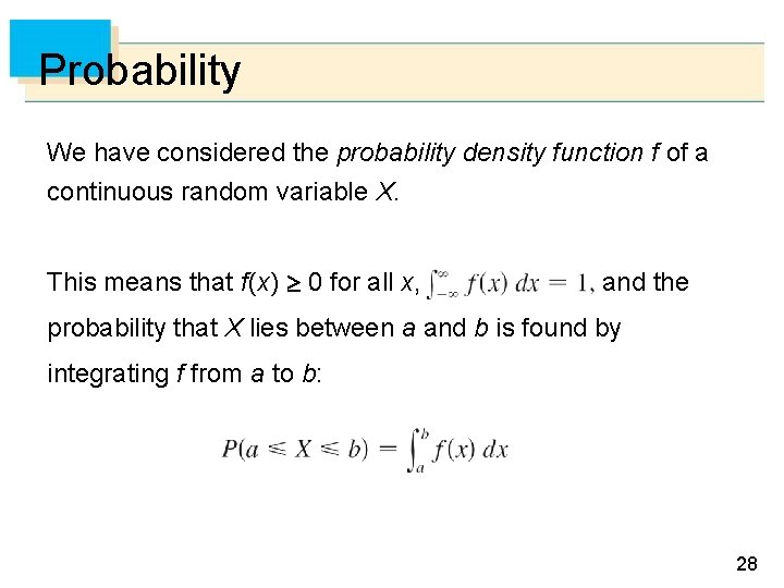
Probability We have considered the probability density function f of a continuous random variable X. This means that f (x) 0 for all x, and the probability that X lies between a and b is found by integrating f from a to b: 28

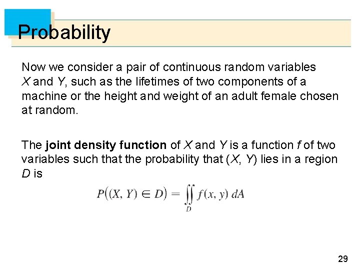
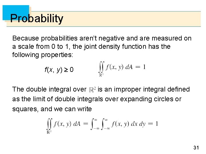
Probability Now we consider a pair of continuous random variables X and Y, such as the lifetimes of two components of a machine or the height and weight of an adult female chosen at random. The joint density function of X and Y is a function f of two variables such that the probability that (X, Y) lies in a region D is 29

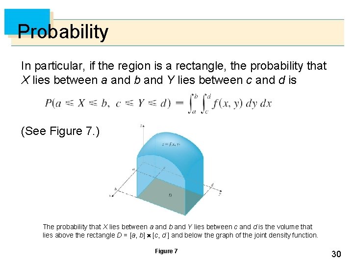
Probability In particular, if the region is a rectangle, the probability that X lies between a and b and Y lies between c and d is (See Figure 7. ) The probability that X lies between a and b and Y lies between c and d is the volume that lies above the rectangle D = [a, b] [c, d ] and below the graph of the joint density function. Figure 7 30

Probability Because probabilities aren’t negative and are measured on a scale from 0 to 1, the joint density function has the following properties: f (x, y) 0 The double integral over is an improper integral defined as the limit of double integrals over expanding circles or squares, and we can write 31

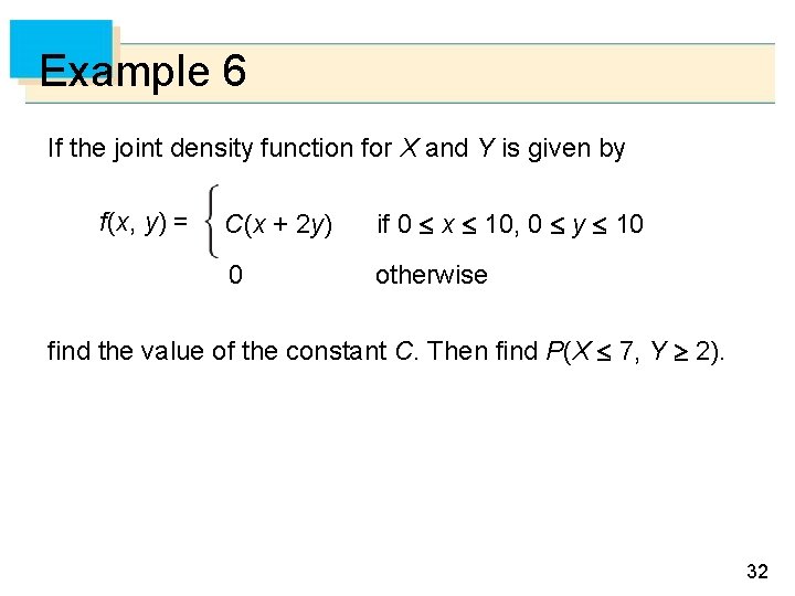
Example 6 If the joint density function for X and Y is given by f (x, y) = C(x + 2 y) if 0 x 10, 0 y 10 0 otherwise find the value of the constant C. Then find P(X 7, Y 2). 32

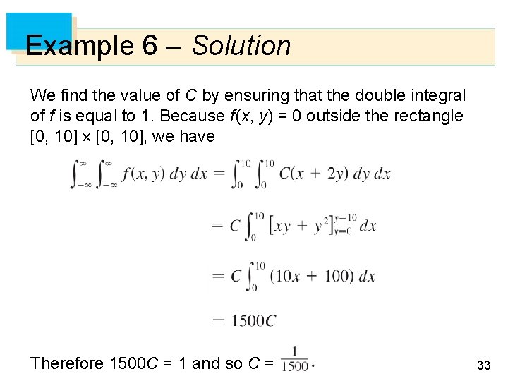
Example 6 – Solution We find the value of C by ensuring that the double integral of f is equal to 1. Because f (x, y) = 0 outside the rectangle [0, 10], we have Therefore 1500 C = 1 and so C = 33

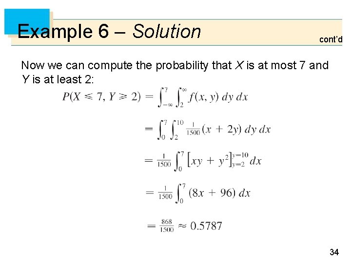
Example 6 – Solution cont’d Now we can compute the probability that X is at most 7 and Y is at least 2: 34

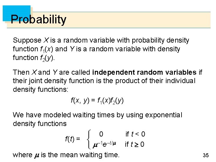
Probability Suppose X is a random variable with probability density function f 1(x) and Y is a random variable with density function f 2(y). Then X and Y are called independent random variables if their joint density function is the product of their individual density functions: f (x, y) = f 1(x)f 2(y) We have modeled waiting times by using exponential density functions 0 if t < 0 f (t) = – 1 e –t / if t 0 where is the mean waiting time. 35

Expected Values 36

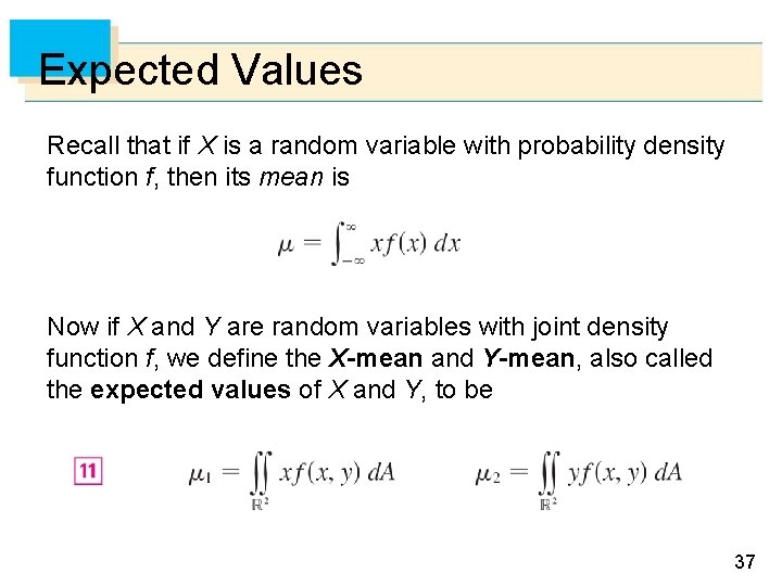
Expected Values Recall that if X is a random variable with probability density function f, then its mean is Now if X and Y are random variables with joint density function f, we define the X-mean and Y-mean, also called the expected values of X and Y, to be 37

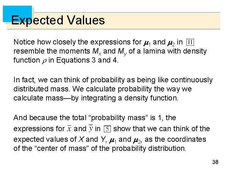
Expected Values Notice how closely the expressions for 1 and 2 in resemble the moments Mx and My of a lamina with density function in Equations 3 and 4. In fact, we can think of probability as being like continuously distributed mass. We calculate probability the way we calculate mass—by integrating a density function. And because the total “probability mass” is 1, the expressions for and in show that we can think of the expected values of X and Y, 1 and 2, as the coordinates of the “center of mass” of the probability distribution. 38

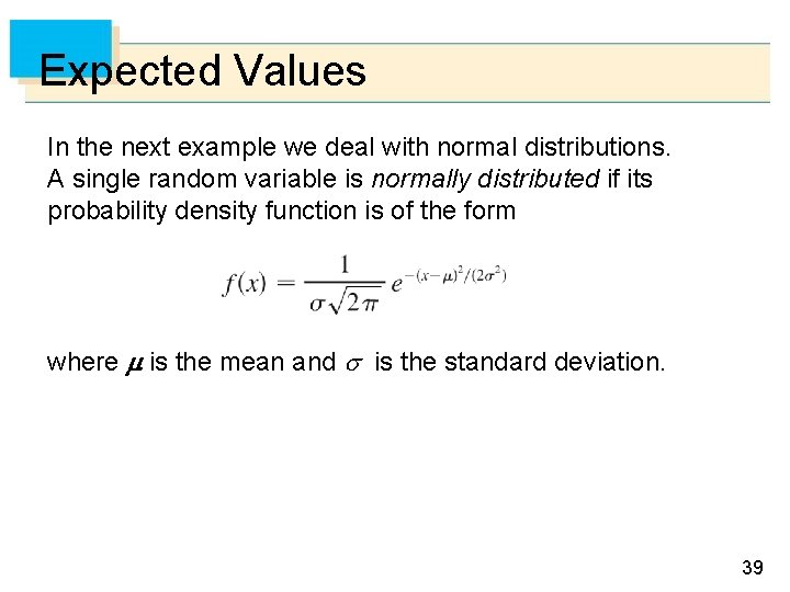
Expected Values In the next example we deal with normal distributions. A single random variable is normally distributed if its probability density function is of the form where is the mean and is the standard deviation. 39

Example 8 A factory produces (cylindrically shaped) roller bearings that are sold as having diameter 4. 0 cm and length 6. 0 cm. In fact, the diameters X are normally distributed with mean 4. 0 cm and standard deviation 0. 01 cm while the lengths Y are normally distributed with mean 6. 0 cm and standard deviation 0. 01 cm. Assuming that X and Y are independent, write the joint density function and graph it. Find the probability that a bearing randomly chosen from the production line has either length or diameter that differs from the mean by more than 0. 02 cm. 40

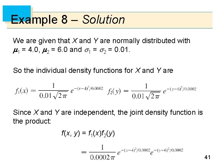
Example 8 – Solution We are given that X and Y are normally distributed with 1 = 4. 0, 2 = 6. 0 and 1 = 2 = 0. 01. So the individual density functions for X and Y are Since X and Y are independent, the joint density function is the product: f (x, y) = f 1(x)f 2(y) 41

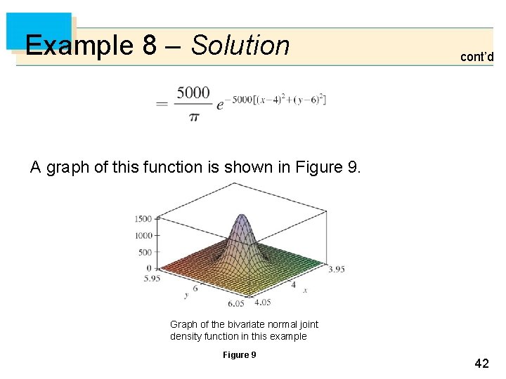
Example 8 – Solution cont’d A graph of this function is shown in Figure 9. Graph of the bivariate normal joint density function in this example Figure 9 42

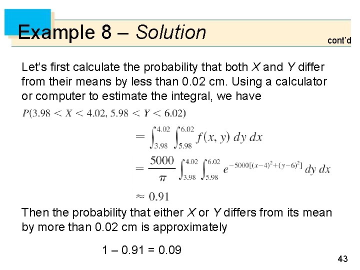
Example 8 – Solution cont’d Let’s first calculate the probability that both X and Y differ from their means by less than 0. 02 cm. Using a calculator or computer to estimate the integral, we have Then the probability that either X or Y differs from its mean by more than 0. 02 cm is approximately 1 – 0. 91 = 0. 09 43