UNIT 4 Radar Receivers The Radar Receiver The

UNIT -4

Radar Receivers The Radar Receiver: • The function of the radar receiver is to detect desired echo signals in the presence of noise, interference, or clutter. • It must separate wanted from unwanted signals, and amplify the wanted signals to a level where target information can be displayed to an operator or used in an automatic data processor. • The design of the radar receiver will depend not only on the type of waveform to be detected, but on the nature of the noise, interference, and clutter echoes with which the desired echo signals must compete. • Noise can enter the receiver via the antenna terminals along with the desired signals, or it might be generated within the receiver itself. • At the microwave frequencies usually used for radar, the external noise which enters via the antenna is generally quite low so that the receiver sensitivity is usually set by the internal noise generated within the receiver. The measure of receiver internal noise is the noise-figure.

• Good receiver design is based on maximizing the output signal-tonoise ratio. • To maximize the output signal-to-noise ratio, the receiver must be designed as a matched filter, or its equivalent. • The matched filter specifies the frequency response function of the IF part of the radar receiver. • Obviously, the receiver should be designed to generate as little internal noise as possible, especially in the input stages where the desired signals are weakest. • Although special attention must be paid to minimize the noise of the input stages, the lowest noise receivers are not always desired in many radar applications if other important receiver properties must be sacrificed.

Noise Figure and Noise Temperature-Derivations Noise Figure: • The noise figure of a receiver was described as a measure of the noise produced by a practical receiver as compared with the noise of an ideal receiver. The noise figure Fn of a linear network may be defined as

• "Available power" refers to the power which would be delivered to a matched load. • The available gain G is equal to Sout/Sin, k = Boltzmann's constant = 1. 38 x 10 -23 J/deg, To =standard temperature of 290 K(approximately room temperature), “B” is the noise bandwidth. The product k. To ≈ 4 x 10 -21 W/Hz. • The purpose for defining a standard temperature is to refer any measurements to a common basis of comparison. Equation above permits two different but equivalent interpretations of noise figure. • It may be considered as the degradation of the signal-to-noise ratio caused by the network (receiver), or it may be interpreted as the ratio of the actual available output noise power to the noise power which would be available if the network merely amplified thermal noise. The noise figure may also be written

• where N is the additional noise introduced by the network itself. The noise figure is commonly expressed in decibels, that is, 10 log Fn. The term noise factor is also used at times instead of noise figure. The two terms are synonymous. • The definition of noise figure assumes the input and output of the network are matched. In some devices less noise is obtained under mismatched, rather than matched, conditions. In spite of definitions, such networks would be operated so as to achieve the maximum output signal-to-noise ratio.

Noise Temperature : • The noise introduced by a network may also be expressed as an effective noise temperature, Te, defined as that (fictional) temperature at the input of the network which would account for the noise N at the output. Therefore N = k Te B n G and • The system noise temperature Ts is defined as the effective noise temperature of the receiver system including the effects of antenna temperature Ta. (It is also sometimes called the system operating noise temperature) If the receiver effective noise temperature is Te, then

• where Fs is the system noise-figure including the effect of antenna temperature. The effective noise temperature of a receiver consisting of a number of networks in cascade is • where Ti and Gi , are the effective noise temperature and gain of the ith network. The effective noise temperature and the noise figure both describe the same characteristic of a network. In general, the effective noise temperature has been preferred for describing low-noise devices, and the noise figure is preferred for conventional receivers.

Radar Displays • The purpose of the display is to visually present in a form suitable for operator interpretation and action the information contained in the radar echo signal. • When the display is connected directly to the video output of the receiver, the information displayed is called raw video. This is the "traditional” type of radar presentation. • When the receiver video output is first processed by an automatic detector or automatic detection and tracking processor (ADT), the output displayed is sometimes called synthetic video. • The cathode-ray tube (CRT) has been almost universally used as the radar display. There are two basic cathode-ray tube displays. One is the deflection-modulated CRT, such as the A-scope, in which a target is indicated by the deflection of the electron beam.

• The other is the intensity modulated CRT, such as the PPI, in which a target is Indicated by intensifying the electron beam and presenting a luminous spot on the face of the CRT. • In general, deflection-modulated displays have the advantage of simpler circuits than those of intensity- modulated displays, and targets may be more readily discerned in the presence of noise or interference. • On the other hand, intensity-modulated displays have the advantage of presenting data in a convenient and easily interpreted form. • The deflection of the beam or the appearance of an intensity-modulated spot on a radar display caused by the presence of a target is commonly referred to as a blip.

Various Types of Radar Displays and its Significance : • The various types of CRT displays which might be used for surveillance and tracking radars are defined as follows : • A-scope: A deflection-modulated display in which the vertical deflection is proportional to target echo strength and the horizontal coordinate is proportional to range. A-scope is similar to synthetic video displays and also known as range scope A-scope is a deflection modulated display and is mostly used for tracking radars • • B-scope: An intensity-modulated rectangular display with azimuth angle indicated by the horizontal coordinate and range by the vertical coordinate. • • • C-scope: An intensity-modulated rectangular display with azimuth angle indicated by the horizontal coordinate and elevation angle by the vertical coordinate It gives direction to the target up and to the right, but not the true range D-scope: A C-scope in which the blips extend vertically to give a rough estimate of distance.

• E-scope: An intensity-modulated rectangular display with distance indicated by the horizontal coordinate and elevation angle by the vertical coordinate. Similar to the B-scope only difference is in E-scope elevation is used instead of azimuth. • F-Scope: A rectangular display in which a target appears as a centralized blip when the radar antenna is aimed at it. Horizontal and vertical aiming errors are respectively indicated by the horizontal and vertical displacement of the blip. • G-Scope: A rectangular display in which a target appears as a laterally centralized blip when the radar antenna is aimed at it in azimuth, and wings appear to grow on the pip as the distance to the target is diminished; horizontal and vertical aiming errors are respectively indicated by horizontal and vertical displacement of the blip. • H-scope: A B-scope modified to include indication of angle of elevation. The target appears as two closely spaced blips which approximate a short bright line, the slope of which is in proportion to the sine of the angle of target elevation.

• I-scope: A display in which a target appears as a complete circle when the radar antenna is pointed at it and in which the radius of the circle is proportional to target distance; incorrect aiming of the antenna changes the circle to a segment whose arc length is inversely proportional to the magnitude of the pointing error, and the position of the segment indicates the reciprocal of the pointing direction of the antenna. • J-scope: A modified A-scope in which the time base is a circle and targets appear as radial deflections from the time base. • K-scope: A modified A-scope in which a target appears as a pair of vertical deflections. When the radar antenna is correctly pointed at the target, the two deflections are of equal height, and when not so pointed, the difference in deflection amplitude is an indication of the direction and magnitude of the pointing error.

• L-scope: A display in which a target appears as two horizontal blips, one extending to the right from a central vertical time base and the other to the left; both blips are of equal amplitude when the radar is pointed directly at the target, any inequality representing relative pointing error, and distance upward along the baseline representing target distance. • M-scope: A type of A-scope in which the target distance is determined by moving an adjustable pedestal signal along the baseline until it coincides with the horizontal position of the target signal deflections; the control which moves the pedestal is calibrated in distance. • N-scope: A K-scope having an adjustable pedestal signal, as in the Mscope, for the measurement of distance. • O-scope: An A-scope modified by the inclusion of an adjustable notch for measuring distance

• PPI or Plan Position Indicator (also called P-scope): An intensitymodulated circular display on which echo signals produced from reflecting objects are shown in plan position with range and azimuth angle displayed in polar (rho-theta) coordinates, forming a map-like display. • An offset, or off center, PPI has the zero position of the time base at a position other than at the center of the display to provide the equivalent of a larger display for a selected portion of the service area. A delayed PPI is one in which the initiation of the time base is delayed. • R-scope: An A-scope with a segment of the time base expanded near the blip for greater accuracy in distance measurement. • RHI or Range-Height Indicator: An intensity modulated display with height (altitude) as the vertical axis and range as the horizontal axis.

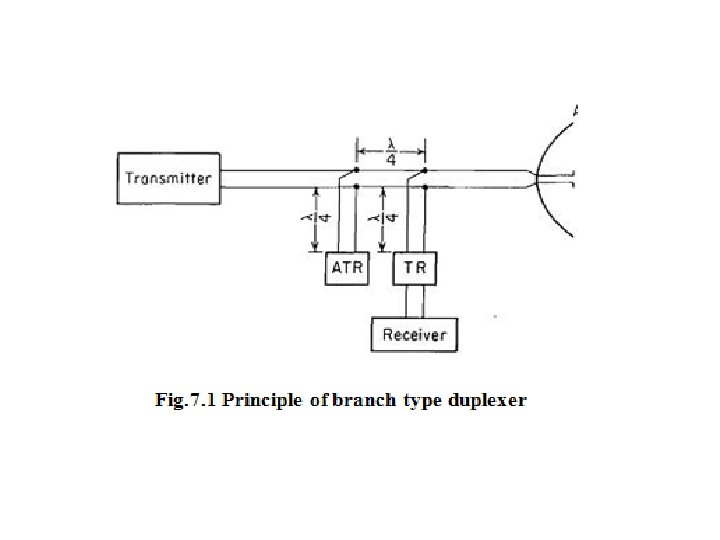
Radar Duplexers Branch type Duplexer : • The branch-type duplexer, diagrammed in Fig. 7. 1 was one of the earliest duplexer configurations employed. It consists of a TR (transmit-receive) switch and an ATR (anti-transmit receive) switch, both of which are gasdischarge tubes. • When the transmitter is turned on, the TR and the ATR tubes ionize; that is, they break down, or fire. The TR in the fired condition acts as a short circuit to prevent transmitter power from entering the receiver. • Since the TR is located a quarter wavelength from the main transmission line, it appears as a short circuit at the receiver but as an open circuit at the transmission line so that it does not impede the flow of transmitter power. • Since the ATR is displaced a quarter wavelength from the main transmission line, the short circuit it produces during the fired condition appears as an open circuit on the transmission line and thus has no effect on transmission.

• During reception, the transmitter is off and neither the TR nor the ATR is fired. The open circuit of the ATR, being a quarter wave from the transmission line, appears as a short circuit across the line. • Since this short circuit is located a quarter wave from the receiver branchline, the transmitter is effectively disconnected from the line and the echo signal power is directed to the receiver. The diagram of Fig. 7. 1 is a parallel configuration. Series or series-parallel configurations are possible. • The branch-type duplexer is of limited bandwidth and power-handling capability, and has generally been replaced by the balanced duplexer and other protection devices. It is used, inspite of these limitations, in some low -cost radars.

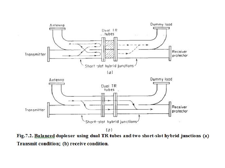
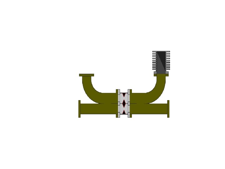
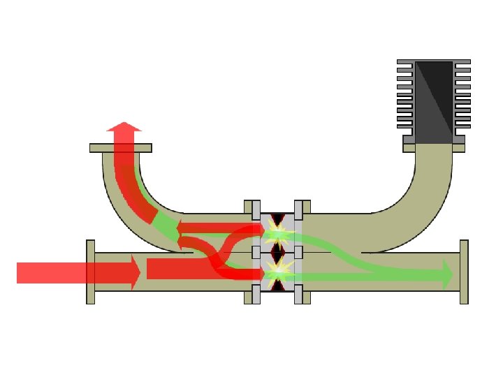
Balanced Type Duplexer • The balanced duplexer, Fig. 7. 2, is based on the short-slot hybrid junction which consists of two sections of waveguides joined along one of their narrow walls with a slot cut in the common narrow wall to provide coupling between the two. • The short-slot hybrid may be considered as a broadband directional coupler with a coupling ratio of 3 d. B. In the transmit condition (Fig. 7. 2 a) power is divided equally into each waveguide by the first short slot hybrid junction. Both TR tubes break down and reflect the incident power out the antenna arm as shown

• The short-slot hybrid has the property that each time the energy passes through the slot in either direction, its phase is advanced 90˚. Therefore, the energy must travel as indicated by the solid lines. • Any energy which leaks through the TR tubes (shown by the dashed lines) is directed to the arm with the matched dummy load and not to the receiver, In addition to the attenuation provided by the TR tubes, the hybrid junctions provide an additional 20 to 30 d. B of isolation. • On reception the TR tubes are unfired and the echo signals pass through the duplexer and into the receiver as shown in Fig. 7. 2 b. The power splits equally at the first junction and because of the 90˚ phase advance on passing through the slot, the energy recombines in the receiving arm and not in the dummy-load arm. • The power-handling capability of the balanced duplexer is inherently greater than that of the branch-type duplexer and it has wide bandwidth, over ten percent with proper design. A receiver protector is usually inserted between the duplexer and the receiver for added protection.

Circulators • The ferrite circulator is a three-or four-port device that can, in principle, offer separation of the transmitter and receiver without the need for the conventional duplexer configurations. The circulator does not provide sufficient protection by itself and requires a receiver protector as in Fig. 8. • The isolation between the transmitter and receiver ports of a circulator is seldom sufficient to protect the receiver from damage. • However, it is not the isolation between transmitter and receiver ports that usually determines the amount of transmitter power at the receiver, but the impedance mismatch at the antenna which reflects transmitter power back into the receiver. • The VSWR is a measure of the amount of power reflected by the antenna. For example, a VSWR of 1. 5 means that about 4 percent of the transmitter power will be reflected by the antenna mismatch in the direction of the receiver, which corresponds to an isolation of only 14 d. B.

• Thus, a receiver protector is almost always required. It also reduces to safe level radiations from nearby transmitters. The receiver protector might use solid-state diodes for an all solid-state configuration, or it might be a passive TR-limiter consisting of a radioactive primed TR-tube followed by a diode limiter. The ferrite circulator with receiver protector is attractive for radar applications because of its long life, wide bandwidth, and compact design.

Radar Antennas Phased Array : • The phased array is a directive antenna made up of individual radiating antennas, or elements, which generate a radiation pattern whose shape and direction is determined by the relative phases and amplitudes of the currents at the individual elements. • By properly varying the relative phases it is possible to steer the direction of the radiation. • The radiating elements might be dipoles open-ended waveguides, slots cut in waveguide, or any other type of antenna. • The inherent flexibility offered by the phased-array antenna in steering the beam by means of electronic control is what has made it of interest for radar. • It has been considered in those radar applications where it is necessary to shift the beam rapidly from one position in space to another, or where it is required to obtain information about many targets at a flexible, rapid data rate.

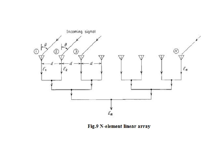
• The full potential of a phased-array antenna requires the use of a computer that can determine in real time, on the basis of the actual operational situation, how best to use the capabilities offered by the array. Radiation pattern for Phased array Antenna : • Consider a linear array made up of N elements equally spaced a distance d apart (Fig. 9). The elements are assumed to be isotropic point sources radiating uniformly in all directions with equal amplitude and phase. Although isotropic elements are not realizable in practice, they are a useful concept in array theory, especially for the computation of radiation patterns. • The array is shown as a receiving antenna for convenience, but because of the reciprocity principle, the results obtained apply equally well to a transmitting antenna. The outputs of all the elements are summed via lines of equal length to give a sum output voltage Ea. • Element 1 will be taken as the reference signal with zero phase. • The difference in the phase of the signals in adjacent elements is Ψ = 2Π (d/λ) sinθ, where θ is the direction of the incoming radiation.

• It is further assumed that the amplitudes and phases of the signals at each element are weighted uniformly. Therefore the amplitudes of the voltages in each element are the same and, for convenience, will be taken to be unity. • The sum of all the voltages from the individual elements, when the phase difference between adjacent elements is Ψ, can be written.

• • • The first factor is a sine wave of frequency ω with a phase shift (N - l)Ψ/2 (if the phase reference were taken at the center of the array, the phase shift would be zero), while the second term represents an amplitude factor of the form sin (NΨ/2)/sin(Ψ/2). The field intensity pattern is the magnitude of the Eq. above The pattern has nulls (zeros) when the numerator is zero. The denominator, however, is zero when Π (d/λ) sinθ, = 0, ± Π, ± 2Π. . . , ± nΠ. Note that when the denominator is zero, the numerator is also zero. The value of the field intensity pattern is indeterminate when both the denominator and numerator are zero. However, by applying L'Hopital's rule it is found that ׀ Ea ׀ is a maximum whenever sinθ = ± nλ/d. These maxima all have the same value and are equal to N. The maximum at sinθ = 0 defines the main beam. The other maxima are called grating lobes.

• From Eq. above, Ea (θ) = Ea (Π - θ). Therefore an antenna of isotropic elements has a similar pattern in the rear of the antenna as in the front. The same would be true for an array of dipoles. • To avoid ambiguities, the backward radiation is usually eliminated by placing a reflecting screen behind the array. Thus only the radiation over the forward half of the antenna (-90˚ ≤ θ ≤ 90°) need be considered. • The radiation pattern is equal to the normalized square of the amplitude, or

• If the spacing between antenna elements is λ/2 and if the sine in the denominator of Eq. above is replaced by its argument, the half-power beamwidth is approximately equal to • The first sidelobe, for N sufficiently large, is 13. 2 d. B be 1 ow the main beam. The pattern of a uniformly illuminated array with elements spaced λ/2 apart is similar to the pattern produced by a continuously illuminated uniform aperture. • When directive elements are used, the resultant array antenna radiation pattern is

• Where Ge (θ) is the radiation pattern of an individual element. The resultant radiation pattern is the product of the element factor Ge(θ) and the array factor Ga(θ), the latter being the pattern of an array composed of isotropic elements. The array factor has also been called the space factor. • Grating lobes caused by a widely spaced array may therefore be eliminated with directive elements which radiate little or no energy in the directions of the undesired lobes

Beam Steering • The beam of an array antenna may be steered rapidly in space without moving large mechanical masses by properly varying the phase of the signals applied to each element. • Consider an array of equally spaced elements. The spacing between adjacent elements is d, and the signals at each element are assumed of equal amplitude. • If the same phase is applied to all elements, the relative phase difference between adjacent elements is zero and the position of the main beam will be broadside to the array at an angle θ = 0. • The main beam will point in a direction other than broadside if the relative phase difference between elements is other than zero. • The direction of the main beam is at an angle θ 0, when the phase difference is Ø = 2π(d/λ) sin θ 0. • The phase at each element is therefore Øc = mØ, where m = 0, 1, 2, ……. . (N 1), and Øc , is any constant phase applied to all elements. • The normalized radiation pattern of the array when the phase difference between adjacent elements is Ø is given by

• The maximum of the radiation pattern occurs when sin θ = sin θo • The above equation states that the main beam of the antenna pattern may be positioned to an angle θ 0 by the insertion of the proper phase shift Ø at each element of the array. • If variable rather than fixed, phase shifters are used, the beam may be steered as the relative phase between elements is changed.

• Using an argument similar to the non scanning array described previously, grating lobes appear at an angle θo whenever the denominator is zero, when • If a grating lobe is permitted to appear at - 90° when the main beam is steered to +90°, it is found from the above that d = λ / 2. • Thus the element spacing must not be larger than a half wavelength the beam is to be steered over a wide angle without having undesirable grating lobes appear. • Practical array antennas do not scan ± 90°. If the scan is limited to ± 60°, the element spacing should be less than 0. 54λ.

Beam Width Changes Change of beamwidth with steering angle: • The half-power beamwidth in the plane of scan increases as the beam is scanned off the broadside direction. The beamwidth is approximately inversely proportional to cosθo, where θo is the angle measured from the normal to the antenna. This may be proved by assuming that the sine in the denominator of Eq. discussed earlier can be replaced by its argument, so that the radiation pattern is of the form • (sin 2 u)/u 2, where u = NΠ (d/λ)(sinθ - sinθo). The (sin 2 u)/u 2 antenna pattern is reduced to half its maximum value when u = ± 0. 443Π. Denote by θ+ the angle corresponding to the half-power point when θ > θo , and θ-, the angle corresponding to the half-power point when θ <θo; that is, θ+ corresponds to u =+0. 443Π and θ- to u = -0. 443Π. • The sinθ - sinθo, term in the expression for u can be written

• The angle between the directions on either side of the main beam of antenna radiation pattern, at which the intensity drops one half of the value is known as antenna beamwidth that is array beam width • It is clear that increase in array physical length results in the decrease in antenna beamwidth for a given propagation wavelength.

• The second term on the right-hand side of Eq. above can be neglected when θo is small (beam is near broadside), so that • Using the above approximation, the two angles corresponding to the 3 -d. B points of the antenna pattern are

• The half-power beamwidth is • Therefore, when the beam is positioned an angle θo off broadside, the beamwidth in the plane of scan increases as (cos θo)-1. The change in beamwidth with angle θo, as derived above is not valid when the antenna beam is too far removed from broadside. It certainly does not apply when the energy is radiated in the end fire direction. • Equation above applies for a uniform aperture illumination. With a cosineon-a-pedestal aperture illumination of the form An = ao + 2 a 1 cos 2Πn/N, the beamwidth is

• The parameter n in the aperture illumination represents the position of the element. Since the illumination is assumed symmetrical about the center element, the parameter n takes on values of n = 0, ± 1, ± 2. . . ± (N - 1)/2. The range of interest is 0 ≤ 2 a 1 ≤ ao which covers the span from uniform illuminations to a taper so severe that the illumination drops to zero at the ends of the array. (The array is assumed to extend a distance d/2 beyond each end element. )

Applications • The phased-array antenna has been of considerable interest to the radar systems engineer because its properties are different from those of other microwave antennas. The array antenna takes several forms: Mechanically scanned array: • The array antenna in this configuration is used to form a fixed beam that is scanned by mechanical motion of the entire antenna. No electronic beam steering is employed. This is an economical approach to air -surveillance radars at the lower radar frequencies, such as VHF. • It is also employed at higher frequencies when a precise aperture illumination is required, as to obtain extremely low sidelobes. • At the lower frequencies, the array might be a collection of dipoles or Yagis, and at the higher frequencies the array might consist of slotted waveguides.

Linear array with frequency scan: • The frequency-scanned, linear array feeding a parabolic cylinder or a planar array of slotted waveguides has seen wide application as a 3 D airsurveillance radar. • In this application, a pencil beam is scanned in elevation by use of frequency and scanned in azimuth by mechanical rotation of the entire antenna. Linear array with phase scan: • Electronic phase steering, instead of frequency scanning, in the 3 D airsurveillance radar is generally more expensive, but allows the use of the frequency domain for purposes other than beam steering. • The linear array configuration is also used to generate multiple, contiguous fixed beams (stacked beams) for 3 D radar. Another application is to use either phase- or frequency-steering in a stationary linear array to steer the beam in one angular coordinate, as for the GCA radar.

Phase-frequency planar array: • A two-dimensional (planar) phased array can utilize frequency scanning to steer the beam in one angular coordinate and phase shifters to steer in the orthogonal coordinate. • This approach is generally easier than using phase shifters to scan in both coordinates, but as with any frequency-scanned array the use of the frequency domain for other purposes is limited when frequency is employed for beam-steering. Phase-phase planar array: • The planar array which utilizes phase shifting to steer the beam in two orthogonal coordinates is the type of array that is of major interest for radar application because of its inherent versatility. • Its application, however, has been limited by its relatively high cost. The phase-phase array is what is generally implied when the term electronically steered phased array is used.

Advantages • The array antenna has the following desirable characteristics not generally enjoyed by other antenna types: Inertia less rapid beam-steering: • The beam from an array can be scanned, or switched from one position to another, in a time limited only by the switching speed of the phase shifters. • Typically, the beam can be switched in several microseconds, but it can be considerably shorter if desired. Multiple, independent beams: • A single aperture can generate many simultaneous independent beams. Alternatively, the same effect can be obtained by rapidly switching a single beam through a sequence of positions. Potential for large peak and / or average power: • If necessary, each element of the array can be fed by a separate high-power transmitter with the combining of the outputs made in space to obtain a total power greater than can be obtained from a single transmitter.

Control of the radiation pattern: • A particular radiation pattern may be more readily obtained with the array than with other microwave antennas since the amplitude and phase of each array element may be individually controlled. • Thus, radiation patterns with extremely low side lobes or with a shaped main beam may be achieved. Separate monopulse sum and difference patterns, each with its own optimum shape, are also possible. Graceful degradation: • The distributed nature of the array means that it can fail gradually rather than all at once (catastrophically). Convenient aperture shape: • The shape of the array permits flush mounting and it can be hardened to resist blast. Electronic beam stabilization: • The ability to steer the beam electronically can be used to stabilize the beam direction when the radar is on a platform, such as a ship or aircraft, that is subject to roll, pitch, or yaw.

Limitations v The major limitation that has limited the widespread use of the conventional phased array in radar is its high cost, which is due in large part to its complexity. v When graceful degradation has gone too far a separate maintenance is needed. v When a planar array is electronically scanned, the change of mutual coupling that accompanies a change in beam position makes the maintenance of low side lobes more difficult. v Although the array has the potential for radiating large power, it is seldom that an array is required to radiate more power than can be radiated by other antenna types or to utilize a total power which cannot possibly be generated by current high-power microwave tube technology that feeds a single transmission line.