Uncertainty wrap up Decision Theory Intro CPSC 322

Uncertainty: wrap up & Decision Theory: Intro CPSC 322 – Decision Theory 1 Textbook § 6. 4. 1 & § 9. 2 March 30, 2011

Remarks on Assignment 4 • Question 2 (Bayesian networks) – “correctly represent the situation described above” means “do not make any independence assumptions that aren’t true” • Step 1: identify the causal network • Step 2: for each network, check if it entails (conditional or marginal) independencies the causal network does not entail. If so, it’s incorrect – Failing to entail some (or all) independencies does not make a network incorrect (only computationally suboptimal) • Question 5 (Rainbow Robot) – If you got rainbowrobot. zip before Sunday, get the updated version: rainbowrobot_updated. zip (on Web. CT) • Question 4 (Decision Networks) – This is mostly Bayes rule and common sense – One could compute the answer algorithmically, but you don’t need to 2

Lecture Overview • • Variable elimination: recap and some more details Variable elimination: pruning irrelevant variables Summary of Reasoning under Uncertainty Decision Theory – Intro – Time-permitting: Single-Stage Decision Problems 3

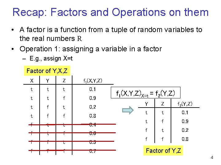
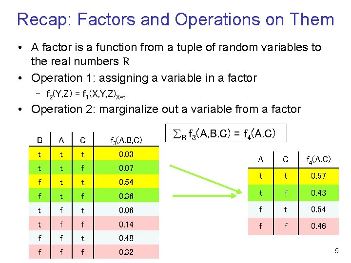
Recap: Factors and Operations on them • A factor is a function from a tuple of random variables to the real numbers R • Operation 1: assigning a variable in a factor – E. g. , assign X=t Factor of Y, X, Z X Y Z f 1(X, Y, Z) t t t 0. 1 t t f 0. 9 t f t 0. 2 t f f 0. 8 f t t 0. 4 f t f 0. 6 f f t 0. 3 f f f 0. 7 f 1(X, Y, Z)X=t = f 2(Y, Z) Y Z f 2(Y, Z) t t 0. 1 t f 0. 9 f t 0. 2 f f 0. 8 Factor of Y, Z 4

Recap: Factors and Operations on Them • A factor is a function from a tuple of random variables to the real numbers R • Operation 1: assigning a variable in a factor – f 2(Y, Z) = f 1(X, Y, Z)X=t • Operation 2: marginalize out a variable from a factor B A C f 3(A, B, C) t t t 0. 03 t t f 0. 07 f t t 0. 54 f t f t B f 3(A, B, C) = f 4(A, C) A C f 4(A, C) t t 0. 57 0. 36 t f 0. 43 t 0. 06 f t 0. 54 f f 0. 14 f f 0. 46 f f t 0. 48 f f f 0. 32 5

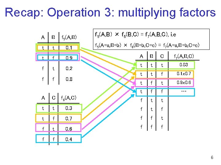
Recap: Operation 3: multiplying factors A B f 5(A, B) t t 0. 1 t f 0. 9 f t 0. 2 f f 0. 8 f 5(A, B) × f 6(B, C) = f 7(A, B, C), i. e f 5(A=a, B=b) × f 6(B=b, C=c) = f 7(A=a, B=b, C=c) A B C f 7(A, B, C) t t t 0. 03 t t f 0. 1 x 0. 7 t f t 0. 9 x 0. 6 t f f … A C f 6(A, C) f t t 0. 3 f t f 0. 7 f f t 0. 6 f f f 0. 4 6

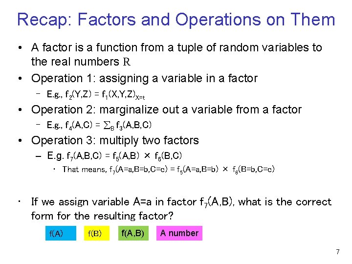
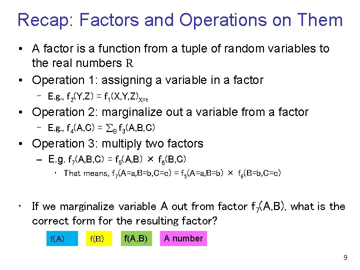
Recap: Factors and Operations on Them • A factor is a function from a tuple of random variables to the real numbers R • Operation 1: assigning a variable in a factor – E. g. , f 2(Y, Z) = f 1(X, Y, Z)X=t • Operation 2: marginalize out a variable from a factor – E. g. , f 4(A, C) = B f 3(A, B, C) • Operation 3: multiply two factors – E. g. f 7(A, B, C) = f 5(A, B) × f 6(B, C) • That means, f 7(A=a, B=b, C=c) = f 5(A=a, B=b) × f 6(B=b, C=c) • If we assign variable A=a in factor f 7(A, B), what is the correct form for the resulting factor? f(A) f(B) f(A, B) A number 7

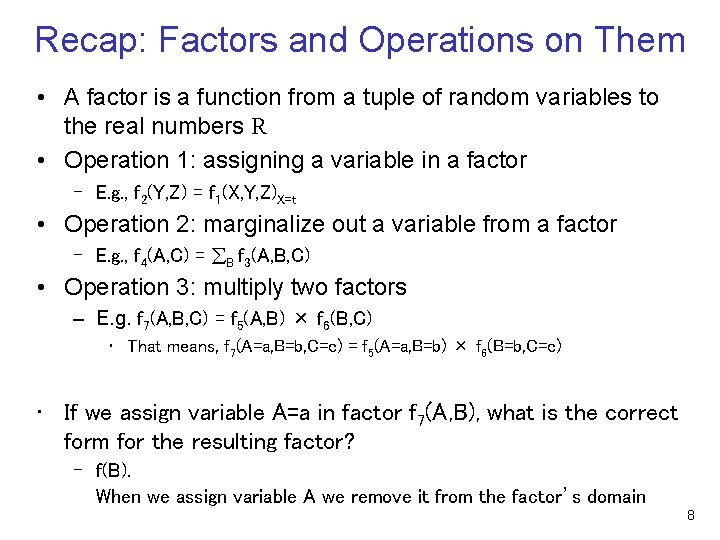
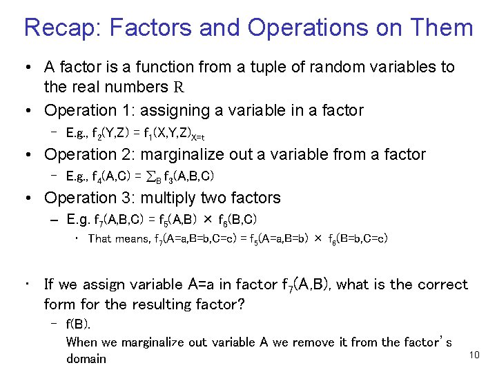
Recap: Factors and Operations on Them • A factor is a function from a tuple of random variables to the real numbers R • Operation 1: assigning a variable in a factor – E. g. , f 2(Y, Z) = f 1(X, Y, Z)X=t • Operation 2: marginalize out a variable from a factor – E. g. , f 4(A, C) = B f 3(A, B, C) • Operation 3: multiply two factors – E. g. f 7(A, B, C) = f 5(A, B) × f 6(B, C) • That means, f 7(A=a, B=b, C=c) = f 5(A=a, B=b) × f 6(B=b, C=c) • If we assign variable A=a in factor f 7(A, B), what is the correct form for the resulting factor? – f(B). When we assign variable A we remove it from the factor’s domain 8

Recap: Factors and Operations on Them • A factor is a function from a tuple of random variables to the real numbers R • Operation 1: assigning a variable in a factor – E. g. , f 2(Y, Z) = f 1(X, Y, Z)X=t • Operation 2: marginalize out a variable from a factor – E. g. , f 4(A, C) = B f 3(A, B, C) • Operation 3: multiply two factors – E. g. f 7(A, B, C) = f 5(A, B) × f 6(B, C) • That means, f 7(A=a, B=b, C=c) = f 5(A=a, B=b) × f 6(B=b, C=c) • If we marginalize variable A out from factor f 7(A, B), what is the correct form for the resulting factor? f(A) f(B) f(A, B) A number 9

Recap: Factors and Operations on Them • A factor is a function from a tuple of random variables to the real numbers R • Operation 1: assigning a variable in a factor – E. g. , f 2(Y, Z) = f 1(X, Y, Z)X=t • Operation 2: marginalize out a variable from a factor – E. g. , f 4(A, C) = B f 3(A, B, C) • Operation 3: multiply two factors – E. g. f 7(A, B, C) = f 5(A, B) × f 6(B, C) • That means, f 7(A=a, B=b, C=c) = f 5(A=a, B=b) × f 6(B=b, C=c) • If we assign variable A=a in factor f 7(A, B), what is the correct form for the resulting factor? – f(B). When we marginalize out variable A we remove it from the factor’s domain 10

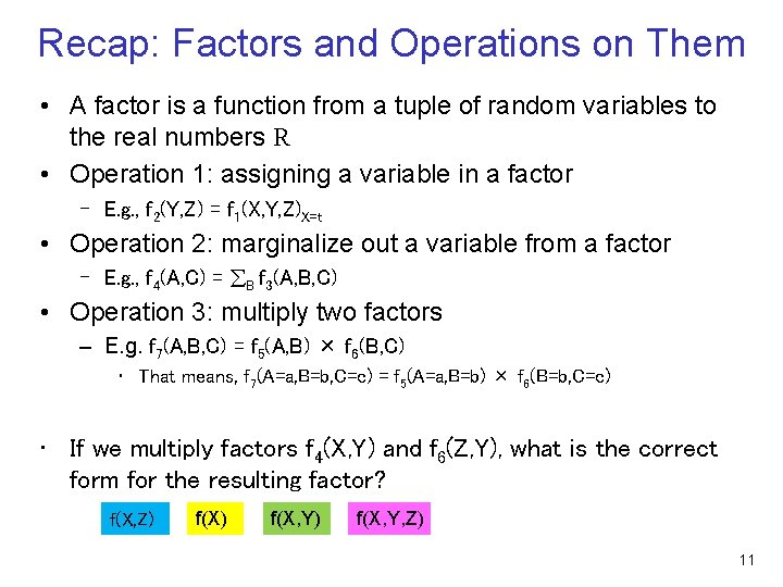
Recap: Factors and Operations on Them • A factor is a function from a tuple of random variables to the real numbers R • Operation 1: assigning a variable in a factor – E. g. , f 2(Y, Z) = f 1(X, Y, Z)X=t • Operation 2: marginalize out a variable from a factor – E. g. , f 4(A, C) = B f 3(A, B, C) • Operation 3: multiply two factors – E. g. f 7(A, B, C) = f 5(A, B) × f 6(B, C) • That means, f 7(A=a, B=b, C=c) = f 5(A=a, B=b) × f 6(B=b, C=c) • If we multiply factors f 4(X, Y) and f 6(Z, Y), what is the correct form for the resulting factor? f(X, Z) f(X, Y) f(X, Y, Z) 11

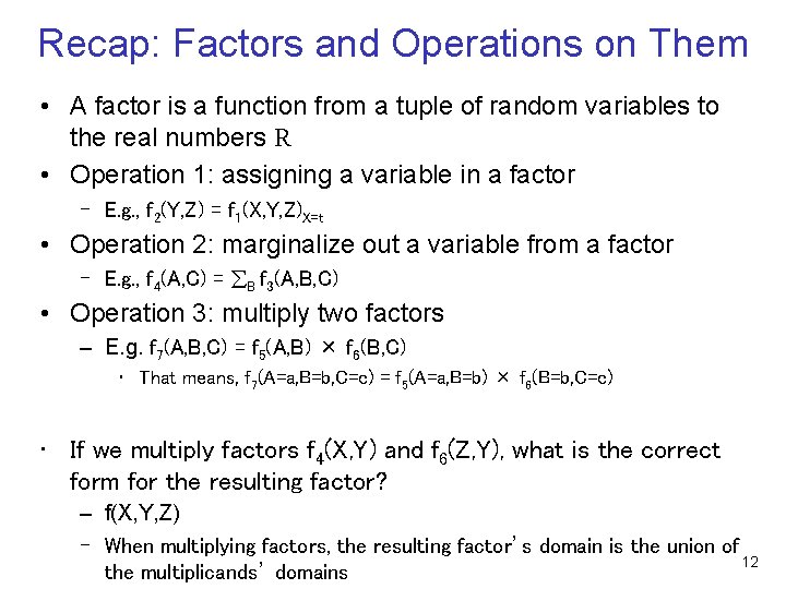
Recap: Factors and Operations on Them • A factor is a function from a tuple of random variables to the real numbers R • Operation 1: assigning a variable in a factor – E. g. , f 2(Y, Z) = f 1(X, Y, Z)X=t • Operation 2: marginalize out a variable from a factor – E. g. , f 4(A, C) = B f 3(A, B, C) • Operation 3: multiply two factors – E. g. f 7(A, B, C) = f 5(A, B) × f 6(B, C) • That means, f 7(A=a, B=b, C=c) = f 5(A=a, B=b) × f 6(B=b, C=c) • If we multiply factors f 4(X, Y) and f 6(Z, Y), what is the correct form for the resulting factor? – f(X, Y, Z) – When multiplying factors, the resulting factor’s domain is the union of 12 the multiplicands’ domains

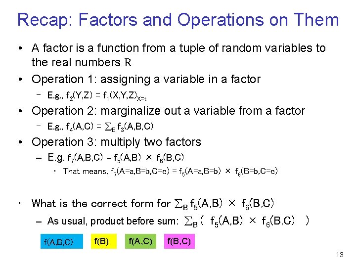
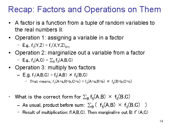
Recap: Factors and Operations on Them • A factor is a function from a tuple of random variables to the real numbers R • Operation 1: assigning a variable in a factor – E. g. , f 2(Y, Z) = f 1(X, Y, Z)X=t • Operation 2: marginalize out a variable from a factor – E. g. , f 4(A, C) = B f 3(A, B, C) • Operation 3: multiply two factors – E. g. f 7(A, B, C) = f 5(A, B) × f 6(B, C) • That means, f 7(A=a, B=b, C=c) = f 5(A=a, B=b) × f 6(B=b, C=c) • What is the correct form for B f 5(A, B) × f 6(B, C) – As usual, product before sum: B ( f 5(A, B) × f 6(B, C) ) f(A, B, C) f(B) f(A, C) f(B, C) 13

Recap: Factors and Operations on Them • A factor is a function from a tuple of random variables to the real numbers R • Operation 1: assigning a variable in a factor – E. g. , f 2(Y, Z) = f 1(X, Y, Z)X=t • Operation 2: marginalize out a variable from a factor – E. g. , f 4(A, C) = B f 3(A, B, C) • Operation 3: multiply two factors – E. g. f 7(A, B, C) = f 5(A, B) × f 6(B, C) • That means, f 7(A=a, B=b, C=c) = f 5(A=a, B=b) × f 6(B=b, C=c) • What is the correct form for B f 5(A, B) × f 6(B, C) – As usual, product before sum: B ( f 5(A, B) × f 6(B, C) ) – Result of multiplication: f(A, B, C). Then marginalize out B: f’(A, C) 14

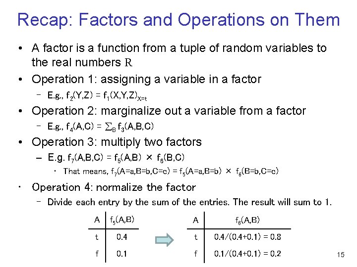
Recap: Factors and Operations on Them • A factor is a function from a tuple of random variables to the real numbers R • Operation 1: assigning a variable in a factor – E. g. , f 2(Y, Z) = f 1(X, Y, Z)X=t • Operation 2: marginalize out a variable from a factor – E. g. , f 4(A, C) = B f 3(A, B, C) • Operation 3: multiply two factors – E. g. f 7(A, B, C) = f 5(A, B) × f 6(B, C) • That means, f 7(A=a, B=b, C=c) = f 5(A=a, B=b) × f 6(B=b, C=c) • Operation 4: normalize the factor – Divide each entry by the sum of the entries. The result will sum to 1. A f 5(A, B) A f 6(A, B) t 0. 4/(0. 4+0. 1) = 0. 8 f 0. 1/(0. 4+0. 1) = 0. 2 15

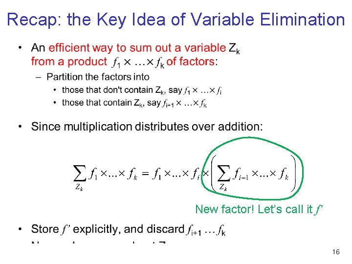
Recap: the Key Idea of Variable Elimination • New factor! Let’s call it f’ 16

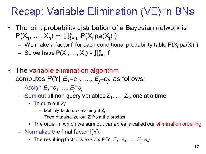
Recap: Variable Elimination (VE) in BNs • 17

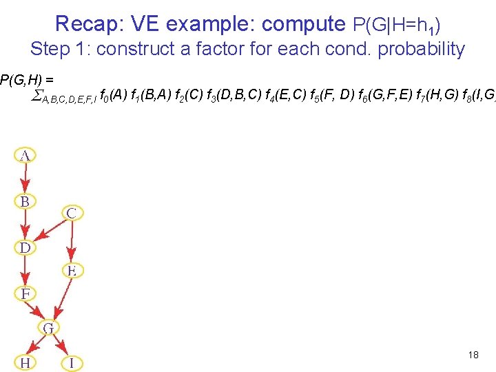
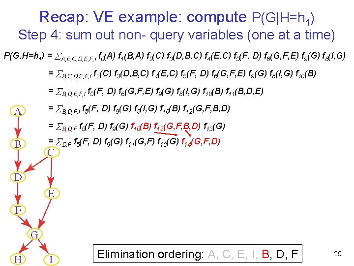
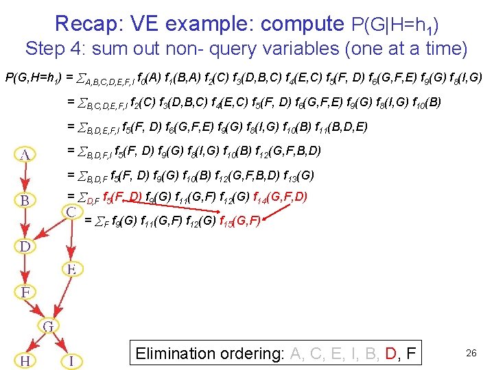
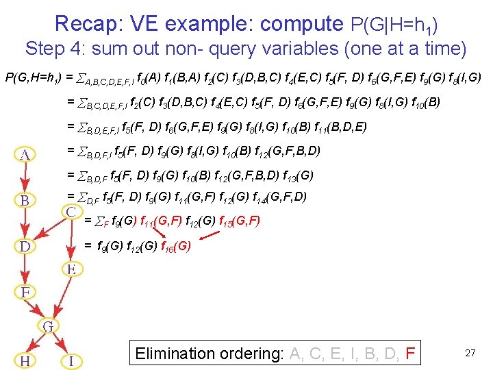
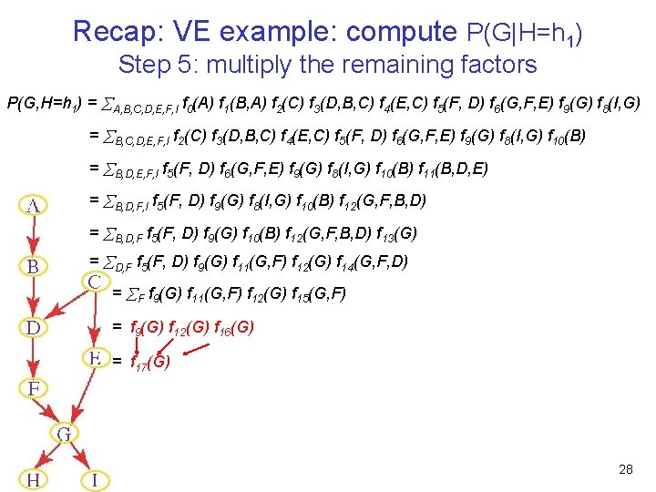
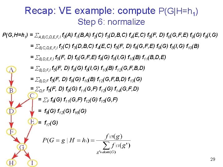
Recap: VE example: compute P(G|H=h 1) Step 1: construct a factor for each cond. probability P(G, H) = A, B, C, D, E, F, I f 0(A) f 1(B, A) f 2(C) f 3(D, B, C) f 4(E, C) f 5(F, D) f 6(G, F, E) f 7(H, G) f 8(I, G) 18

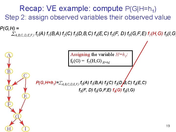
Recap: VE example: compute P(G|H=h 1) Step 2: assign observed variables their observed value P(G, H) = A, B, C, D, E, F, I f 0(A) f 1(B, A) f 2(C) f 3(D, B, C) f 4(E, C) f 5(F, D) f 6(G, F, E) f 7(H, G) f 8(I, G) Assigning the variable H=h 1: f 9(G) = f 7(H, G) H=h 1 P(G, H=h 1)= A, B, C, D, E, F, I f 0(A) f 1(B, A) f 2(C) f 3(D, B, C) f 4(E, C) f 5(F, D) f 6(G, F, E) f 9(G) f 8(I, G) 19

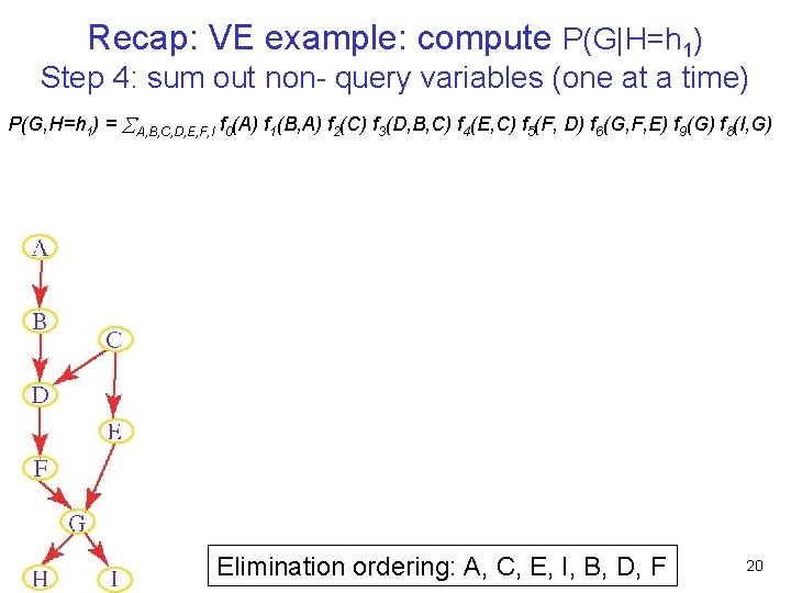
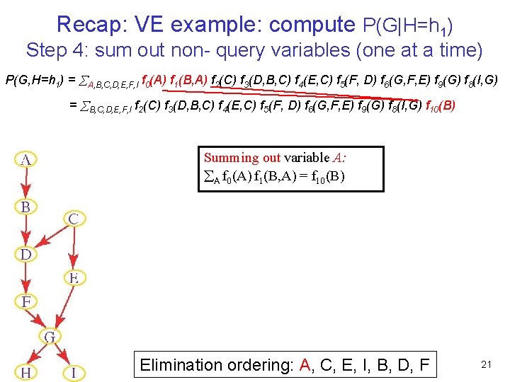
Recap: VE example: compute P(G|H=h 1) Step 4: sum out non- query variables (one at a time) P(G, H=h 1) = A, B, C, D, E, F, I f 0(A) f 1(B, A) f 2(C) f 3(D, B, C) f 4(E, C) f 5(F, D) f 6(G, F, E) f 9(G) f 8(I, G) Elimination ordering: A, C, E, I, B, D, F 20

Recap: VE example: compute P(G|H=h 1) Step 4: sum out non- query variables (one at a time) P(G, H=h 1) = A, B, C, D, E, F, I f 0(A) f 1(B, A) f 2(C) f 3(D, B, C) f 4(E, C) f 5(F, D) f 6(G, F, E) f 9(G) f 8(I, G) = B, C, D, E, F, I f 2(C) f 3(D, B, C) f 4(E, C) f 5(F, D) f 6(G, F, E) f 9(G) f 8(I, G) f 10(B) Summing out variable A: A f 0(A) f 1(B, A) = f 10(B) Elimination ordering: A, C, E, I, B, D, F 21

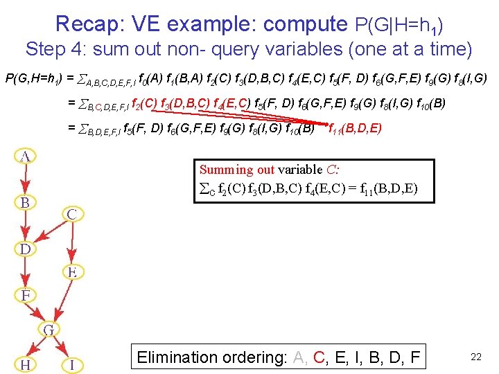
Recap: VE example: compute P(G|H=h 1) Step 4: sum out non- query variables (one at a time) P(G, H=h 1) = A, B, C, D, E, F, I f 0(A) f 1(B, A) f 2(C) f 3(D, B, C) f 4(E, C) f 5(F, D) f 6(G, F, E) f 9(G) f 8(I, G) = B, C, D, E, F, I f 2(C) f 3(D, B, C) f 4(E, C) f 5(F, D) f 6(G, F, E) f 9(G) f 8(I, G) f 10(B) = B, D, E, F, I f 5(F, D) f 6(G, F, E) f 9(G) f 8(I, G) f 10(B) f 11(B, D, E) Summing out variable C: C f 2(C) f 3(D, B, C) f 4(E, C) = f 11(B, D, E) Elimination ordering: A, C, E, I, B, D, F 22

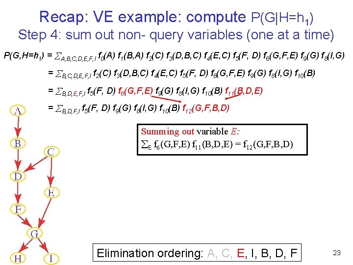
Recap: VE example: compute P(G|H=h 1) Step 4: sum out non- query variables (one at a time) P(G, H=h 1) = A, B, C, D, E, F, I f 0(A) f 1(B, A) f 2(C) f 3(D, B, C) f 4(E, C) f 5(F, D) f 6(G, F, E) f 9(G) f 8(I, G) = B, C, D, E, F, I f 2(C) f 3(D, B, C) f 4(E, C) f 5(F, D) f 6(G, F, E) f 9(G) f 8(I, G) f 10(B) = B, D, E, F, I f 5(F, D) f 6(G, F, E) f 9(G) f 8(I, G) f 10(B) f 11(B, D, E) = B, D, F, I f 5(F, D) f 9(G) f 8(I, G) f 10(B) f 12(G, F, B, D) Summing out variable E: E f 6(G, F, E) f 11(B, D, E) = f 12(G, F, B, D) Elimination ordering: A, C, E, I, B, D, F 23

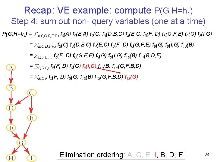
Recap: VE example: compute P(G|H=h 1) Step 4: sum out non- query variables (one at a time) P(G, H=h 1) = A, B, C, D, E, F, I f 0(A) f 1(B, A) f 2(C) f 3(D, B, C) f 4(E, C) f 5(F, D) f 6(G, F, E) f 9(G) f 8(I, G) = B, C, D, E, F, I f 2(C) f 3(D, B, C) f 4(E, C) f 5(F, D) f 6(G, F, E) f 9(G) f 8(I, G) f 10(B) = B, D, E, F, I f 5(F, D) f 6(G, F, E) f 9(G) f 8(I, G) f 10(B) f 11(B, D, E) = B, D, F, I f 5(F, D) f 9(G) f 8(I, G) f 10(B) f 12(G, F, B, D) = B, D, F f 5(F, D) f 9(G) f 10(B) f 12(G, F, B, D) f 13(G) Elimination ordering: A, C, E, I, B, D, F 24

Recap: VE example: compute P(G|H=h 1) Step 4: sum out non- query variables (one at a time) P(G, H=h 1) = A, B, C, D, E, F, I f 0(A) f 1(B, A) f 2(C) f 3(D, B, C) f 4(E, C) f 5(F, D) f 6(G, F, E) f 9(G) f 8(I, G) = B, C, D, E, F, I f 2(C) f 3(D, B, C) f 4(E, C) f 5(F, D) f 6(G, F, E) f 9(G) f 8(I, G) f 10(B) = B, D, E, F, I f 5(F, D) f 6(G, F, E) f 9(G) f 8(I, G) f 10(B) f 11(B, D, E) = B, D, F, I f 5(F, D) f 9(G) f 8(I, G) f 10(B) f 12(G, F, B, D) = B, D, F f 5(F, D) f 9(G) f 10(B) f 12(G, F, B, D) f 13(G) = D, F f 5(F, D) f 9(G) f 11(G, F) f 12(G) f 14(G, F, D) Elimination ordering: A, C, E, I, B, D, F 25

Recap: VE example: compute P(G|H=h 1) Step 4: sum out non- query variables (one at a time) P(G, H=h 1) = A, B, C, D, E, F, I f 0(A) f 1(B, A) f 2(C) f 3(D, B, C) f 4(E, C) f 5(F, D) f 6(G, F, E) f 9(G) f 8(I, G) = B, C, D, E, F, I f 2(C) f 3(D, B, C) f 4(E, C) f 5(F, D) f 6(G, F, E) f 9(G) f 8(I, G) f 10(B) = B, D, E, F, I f 5(F, D) f 6(G, F, E) f 9(G) f 8(I, G) f 10(B) f 11(B, D, E) = B, D, F, I f 5(F, D) f 9(G) f 8(I, G) f 10(B) f 12(G, F, B, D) = B, D, F f 5(F, D) f 9(G) f 10(B) f 12(G, F, B, D) f 13(G) = D, F f 5(F, D) f 9(G) f 11(G, F) f 12(G) f 14(G, F, D) = F f 9(G) f 11(G, F) f 12(G) f 15(G, F) Elimination ordering: A, C, E, I, B, D, F 26

Recap: VE example: compute P(G|H=h 1) Step 4: sum out non- query variables (one at a time) P(G, H=h 1) = A, B, C, D, E, F, I f 0(A) f 1(B, A) f 2(C) f 3(D, B, C) f 4(E, C) f 5(F, D) f 6(G, F, E) f 9(G) f 8(I, G) = B, C, D, E, F, I f 2(C) f 3(D, B, C) f 4(E, C) f 5(F, D) f 6(G, F, E) f 9(G) f 8(I, G) f 10(B) = B, D, E, F, I f 5(F, D) f 6(G, F, E) f 9(G) f 8(I, G) f 10(B) f 11(B, D, E) = B, D, F, I f 5(F, D) f 9(G) f 8(I, G) f 10(B) f 12(G, F, B, D) = B, D, F f 5(F, D) f 9(G) f 10(B) f 12(G, F, B, D) f 13(G) = D, F f 5(F, D) f 9(G) f 11(G, F) f 12(G) f 14(G, F, D) = F f 9(G) f 11(G, F) f 12(G) f 15(G, F) = f 9(G) f 12(G) f 16(G) Elimination ordering: A, C, E, I, B, D, F 27

Recap: VE example: compute P(G|H=h 1) Step 5: multiply the remaining factors P(G, H=h 1) = A, B, C, D, E, F, I f 0(A) f 1(B, A) f 2(C) f 3(D, B, C) f 4(E, C) f 5(F, D) f 6(G, F, E) f 9(G) f 8(I, G) = B, C, D, E, F, I f 2(C) f 3(D, B, C) f 4(E, C) f 5(F, D) f 6(G, F, E) f 9(G) f 8(I, G) f 10(B) = B, D, E, F, I f 5(F, D) f 6(G, F, E) f 9(G) f 8(I, G) f 10(B) f 11(B, D, E) = B, D, F, I f 5(F, D) f 9(G) f 8(I, G) f 10(B) f 12(G, F, B, D) = B, D, F f 5(F, D) f 9(G) f 10(B) f 12(G, F, B, D) f 13(G) = D, F f 5(F, D) f 9(G) f 11(G, F) f 12(G) f 14(G, F, D) = F f 9(G) f 11(G, F) f 12(G) f 15(G, F) = f 9(G) f 12(G) f 16(G) = f 17(G) 28

Recap: VE example: compute P(G|H=h 1) Step 6: normalize P(G, H=h 1) = A, B, C, D, E, F, I f 0(A) f 1(B, A) f 2(C) f 3(D, B, C) f 4(E, C) f 5(F, D) f 6(G, F, E) f 9(G) f 8(I, G) = B, C, D, E, F, I f 2(C) f 3(D, B, C) f 4(E, C) f 5(F, D) f 6(G, F, E) f 9(G) f 8(I, G) f 10(B) = B, D, E, F, I f 5(F, D) f 6(G, F, E) f 9(G) f 8(I, G) f 10(B) f 11(B, D, E) = B, D, F, I f 5(F, D) f 9(G) f 8(I, G) f 10(B) f 12(G, F, B, D) = B, D, F f 5(F, D) f 9(G) f 10(B) f 12(G, F, B, D) f 13(G) = D, F f 5(F, D) f 9(G) f 11(G, F) f 12(G) f 14(G, F, D) = F f 9(G) f 11(G, F) f 12(G) f 15(G, F) = f 9(G) f 12(G) f 16(G) = f 17(G) 29

Lecture Overview • • Variable elimination: recap and some more details Variable elimination: pruning irrelevant variables Summary of Reasoning under Uncertainty Decision Theory – Intro – Time-permitting: Single-Stage Decision Problems 30

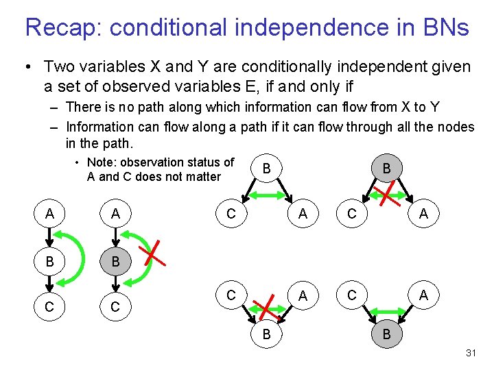
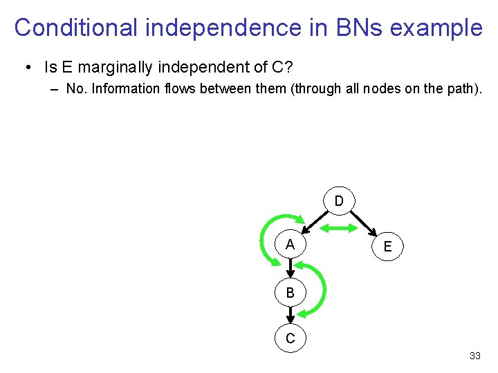
Recap: conditional independence in BNs • Two variables X and Y are conditionally independent given a set of observed variables E, if and only if – There is no path along which information can flow from X to Y – Information can flow along a path if it can flow through all the nodes in the path. • Note: observation status of A and C does not matter A A B B C C B B C A C A B B 31

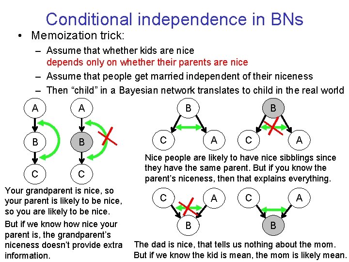
Conditional independence in BNs • Memoization trick: – Assume that whether kids are nice depends only on whether their parents are nice – Assume that people get married independent of their niceness – Then “child” in a Bayesian network translates to child in the real world A A B B C C Your grandparent is nice, so your parent is likely to be nice, so you are likely to be nice. But if we know how nice your parent is, the grandparent’s niceness doesn’t provide extra information. B C B A C A Nice people are likely to have nice sibblings since they have the same parent. But if you know the parent’s niceness, then that explains everything. C A B The dad is nice, that tells us nothing about the mom. But if we know the kid is mean, the mom is likely mean.

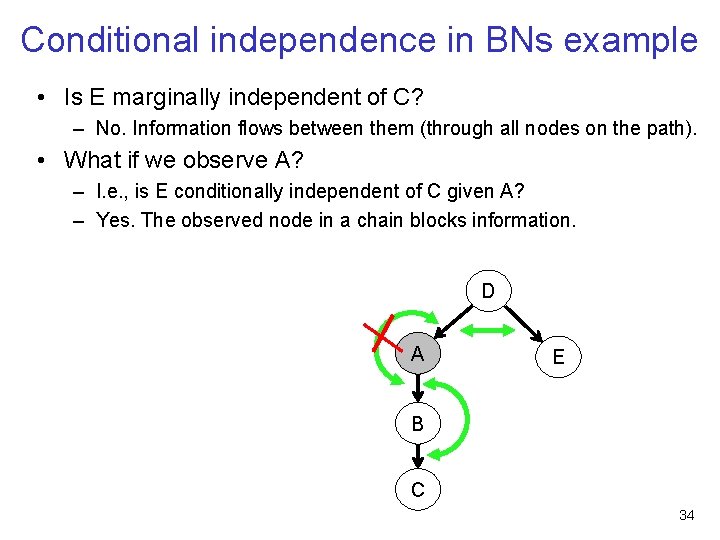
Conditional independence in BNs example • Is E marginally independent of C? – No. Information flows between them (through all nodes on the path). D A E B C 33

Conditional independence in BNs example • Is E marginally independent of C? – No. Information flows between them (through all nodes on the path). • What if we observe A? – I. e. , is E conditionally independent of C given A? – Yes. The observed node in a chain blocks information. D A E B C 34

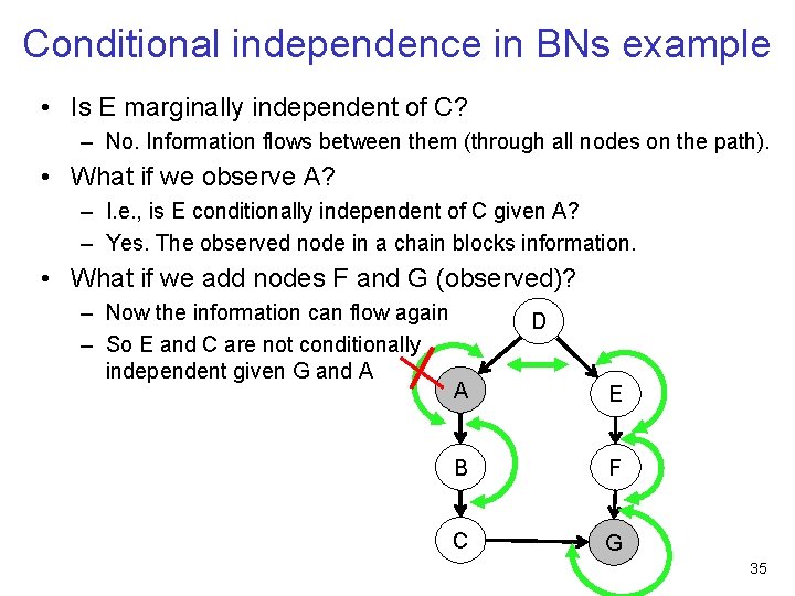
Conditional independence in BNs example • Is E marginally independent of C? – No. Information flows between them (through all nodes on the path). • What if we observe A? – I. e. , is E conditionally independent of C given A? – Yes. The observed node in a chain blocks information. • What if we add nodes F and G (observed)? – Now the information can flow again – So E and C are not conditionally independent given G and A D A E B F C G 35

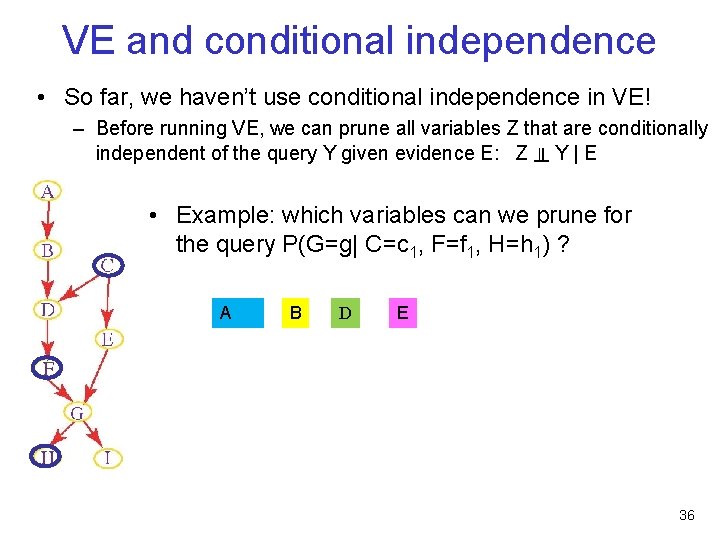
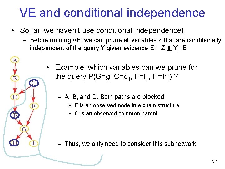
VE and conditional independence • So far, we haven’t use conditional independence in VE! – Before running VE, we can prune all variables Z that are conditionally independent of the query Y given evidence E: Z ╨ Y | E • Example: which variables can we prune for the query P(G=g| C=c 1, F=f 1, H=h 1) ? A B D E 36

VE and conditional independence • So far, we haven’t use conditional independence! – Before running VE, we can prune all variables Z that are conditionally independent of the query Y given evidence E: Z ╨ Y | E • Example: which variables can we prune for the query P(G=g| C=c 1, F=f 1, H=h 1) ? – A, B, and D. Both paths are blocked • F is an observed node in a chain structure • C is an observed common parent – Thus, we only need to consider this subnetwork 37

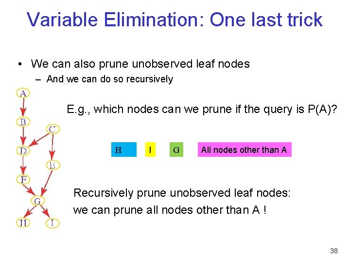
Variable Elimination: One last trick • We can also prune unobserved leaf nodes – And we can do so recursively • E. g. , which nodes can we prune if the query is P(A)? H • • I G All nodes other than A Recursively prune unobserved leaf nodes: we can prune all nodes other than A ! 38

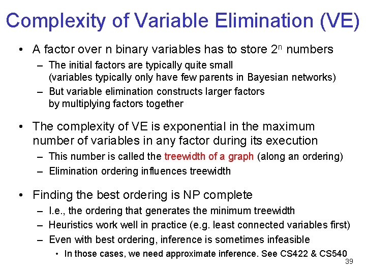
Complexity of Variable Elimination (VE) • A factor over n binary variables has to store 2 n numbers – The initial factors are typically quite small (variables typically only have few parents in Bayesian networks) – But variable elimination constructs larger factors by multiplying factors together • The complexity of VE is exponential in the maximum number of variables in any factor during its execution – This number is called the treewidth of a graph (along an ordering) – Elimination ordering influences treewidth • Finding the best ordering is NP complete – I. e. , the ordering that generates the minimum treewidth – Heuristics work well in practice (e. g. least connected variables first) – Even with best ordering, inference is sometimes infeasible • In those cases, we need approximate inference. See CS 422 & CS 540 39

Lecture Overview • • Variable elimination: recap and some more details Variable elimination: pruning irrelevant variables Summary of Reasoning under Uncertainty Decision Theory – Intro – Time-permitting: Single-Stage Decision Problems 40

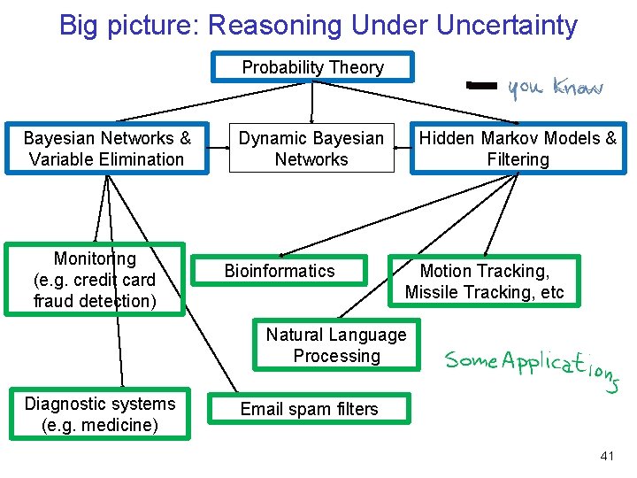
Big picture: Reasoning Under Uncertainty Probability Theory Bayesian Networks & Variable Elimination Monitoring (e. g. credit card fraud detection) Dynamic Bayesian Networks Bioinformatics Hidden Markov Models & Filtering Motion Tracking, Missile Tracking, etc Natural Language Processing Diagnostic systems (e. g. medicine) Email spam filters 41

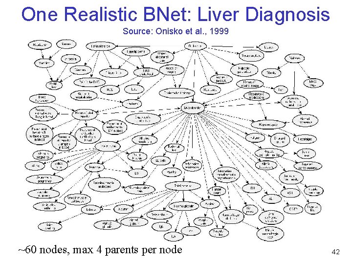
One Realistic BNet: Liver Diagnosis Source: Onisko et al. , 1999 ~60 nodes, max 4 parents per node 42

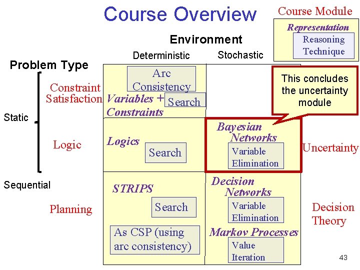
Course Overview Course Module Environment Problem Type Static Deterministic Stochastic Arc Consistency Constraint Satisfaction Variables + Search Constraints Logic Sequential Planning Logics Representation Reasoning Technique This concludes the uncertainty module Bayesian Networks Search Variable Elimination Uncertainty Decision Networks STRIPS Search As CSP (using arc consistency) Variable Elimination Markov Processes Value Iteration Decision Theory 43

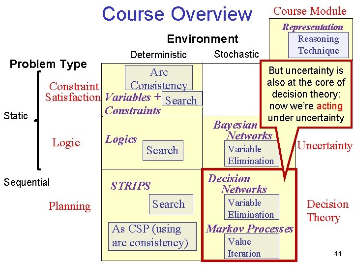
Course Overview Course Module Representation Reasoning Technique Environment Problem Type Static Deterministic Stochastic But uncertainty is also at the core of decision theory: now we’re acting under uncertainty Arc Consistency Constraint Satisfaction Variables + Search Constraints Logic Sequential Planning Logics Bayesian Networks Search Variable Elimination Uncertainty Decision Networks STRIPS Search As CSP (using arc consistency) Variable Elimination Markov Processes Value Iteration Decision Theory 44

Lecture Overview • • Variable elimination: recap and some more details Variable elimination: pruning irrelevant variables Summary of Reasoning under Uncertainty Decision Theory – Intro – Time-permitting: Single-Stage Decision Problems 45

Decisions Under Uncertainty: Intro • Earlier in the course, we focused on decision making in deterministic domains – Search/CSPs: single-stage decisions – Planning: sequential decisions • Now we face stochastic domains – so far we've considered how to represent and update beliefs – What if an agent has to make decisions under uncertainty? • Making decisions under uncertainty is important – We mainly represent the world probabilistically so we can use our beliefs as the basis for making decisions 46

Decisions Under Uncertainty: Intro • An agent's decision will depend on – What actions are available – What beliefs the agent has – Which goals the agent has • Differences between deterministic and stochastic setting – Obvious difference in representation: need to represent our uncertain beliefs – Now we'll speak about representing actions and goals • Actions will be pretty straightforward: decision variables • Goals will be interesting: we'll move from all-or-nothing goals to a richer notion: rating how happy the agent is in different situations. • Putting these together, we'll extend Bayesian networks to make a new representation called decision networks 47

Lecture Overview • • Variable elimination: recap and some more details Variable elimination: pruning irrelevant variables Summary of Reasoning under Uncertainty Decision Theory – Intro – Time-permitting: Single-Stage Decision Problems 48

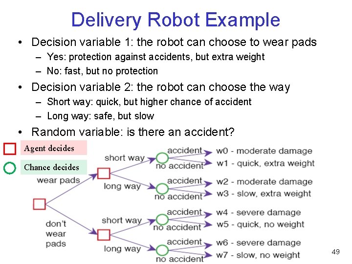
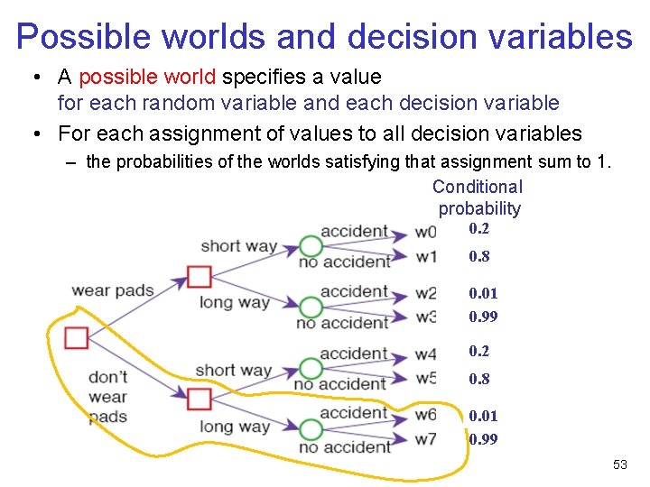
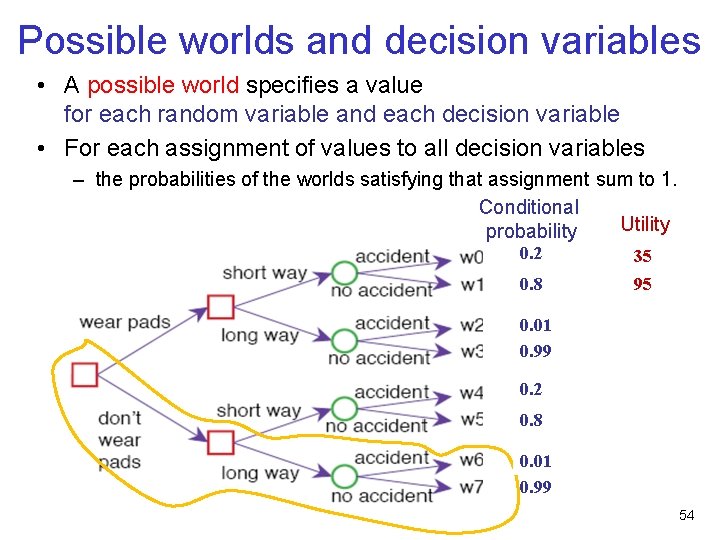
Delivery Robot Example • Decision variable 1: the robot can choose to wear pads – Yes: protection against accidents, but extra weight – No: fast, but no protection • Decision variable 2: the robot can choose the way – Short way: quick, but higher chance of accident – Long way: safe, but slow • Random variable: is there an accident? Agent decides Chance decides 49

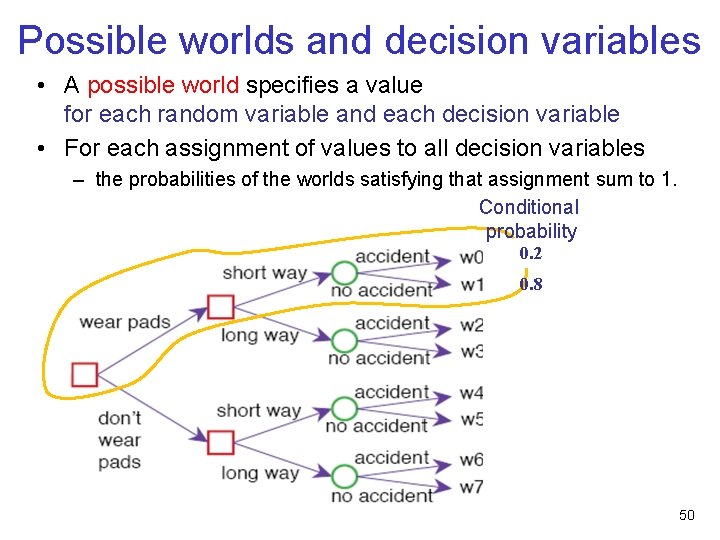
Possible worlds and decision variables • A possible world specifies a value for each random variable and each decision variable • For each assignment of values to all decision variables – the probabilities of the worlds satisfying that assignment sum to 1. Conditional probability 0. 2 0. 8 50

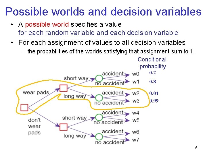
Possible worlds and decision variables • A possible world specifies a value for each random variable and each decision variable • For each assignment of values to all decision variables – the probabilities of the worlds satisfying that assignment sum to 1. Conditional probability 0. 2 0. 8 0. 01 0. 99 51

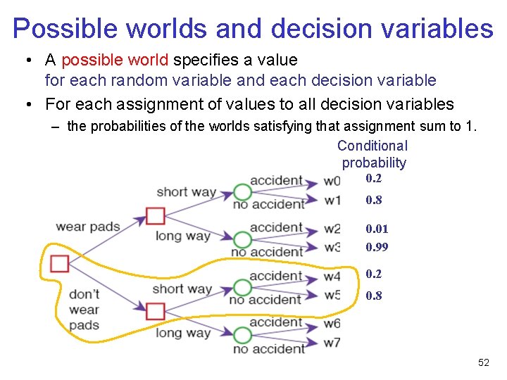
Possible worlds and decision variables • A possible world specifies a value for each random variable and each decision variable • For each assignment of values to all decision variables – the probabilities of the worlds satisfying that assignment sum to 1. Conditional probability 0. 2 0. 8 0. 01 0. 99 0. 2 0. 8 52

Possible worlds and decision variables • A possible world specifies a value for each random variable and each decision variable • For each assignment of values to all decision variables – the probabilities of the worlds satisfying that assignment sum to 1. Conditional probability 0. 2 0. 8 0. 01 0. 99 53

Possible worlds and decision variables • A possible world specifies a value for each random variable and each decision variable • For each assignment of values to all decision variables – the probabilities of the worlds satisfying that assignment sum to 1. Conditional Utility probability 0. 2 35 0. 8 95 0. 01 0. 99 0. 2 0. 8 0. 01 0. 99 54

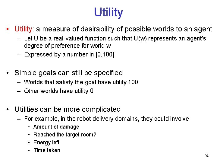
Utility • Utility: a measure of desirability of possible worlds to an agent – Let U be a real-valued function such that U(w) represents an agent's degree of preference for world w – Expressed by a number in [0, 100] • Simple goals can still be specified – Worlds that satisfy the goal have utility 100 – Other worlds have utility 0 • Utilities can be more complicated – For example, in the robot delivery domains, they could involve • • Amount of damage Reached the target room? Energy left Time taken 55

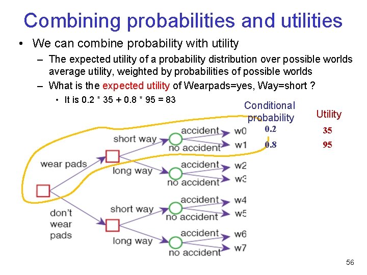
Combining probabilities and utilities • We can combine probability with utility – The expected utility of a probability distribution over possible worlds average utility, weighted by probabilities of possible worlds – What is the expected utility of Wearpads=yes, Way=short ? • It is 0. 2 * 35 + 0. 8 * 95 = 83 Conditional probability Utility 0. 2 35 0. 8 95 56

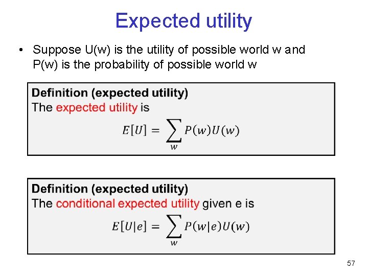
Expected utility • Suppose U(w) is the utility of possible world w and P(w) is the probability of possible world w 57

Expected utility of a decision • Conditional probability Utility E[U|D] 0. 2 35 0. 8 95 0. 01 0. 99 30 35 0. 2 35 3 0. 8 100 0. 01 0. 99 35 0 75 80 83 74. 55 80. 6 79. 2 58

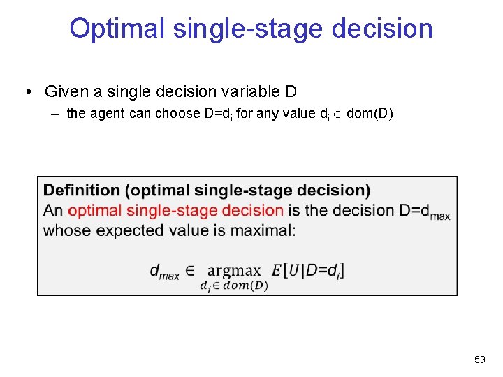
Optimal single-stage decision • Given a single decision variable D – the agent can choose D=di for any value di dom(D) 59

Learning Goals For Today’s Class • Identify implied (in)dependencies in the network • Variable elimination – Carry out variable elimination by using factor representation and using the factor operations – Use techniques to simplify variable elimination • Define a Utility Function on possible worlds • Define and compute optimal one-off decisions • Assignment 4 is due on Monday – You should now be able to solve Questions 1, 2, 3, and 5 – And basically Question 4 • Final exam: Monday, April 11 60