TPOS 202 Western Pacific Workshop The model development

TPOS 202: Western Pacific Workshop The model development activities at FIO Fangli Qiao, Zhenya Song, Qi Shu, Biao Zhao, Guansuo Wang First Institute of Oceanography, SOA, China 4 -6 Sep, 2017 Qingdao, P R China qiaofl@fio. org. cn

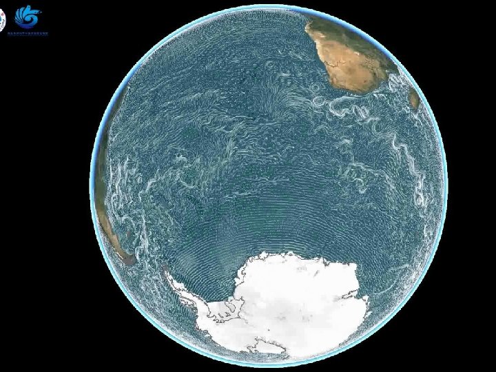
Outlines 1. Challenges faced 2. Surface wave-induced vertical mixing 3. Surface wave in OGCM 4. Surface wave in Typhoon model 5. Surface wave in climate system 6. Discussion and suggestions

1. Challenges faced

Long-standing challenges for OGCM models: Simulated SST is overheating in summertime, and mixed layer depth is too shallow (Martin 1985; Kantha 1994; Ezer 2000; Mellor 2003; Qiao etal, 2016). Long-standing challenges for Typhoon models: Typhoon/ Hurricane intensity. Long-standing challenges for climate models: Tropical bias such as too cold tongue in tropical Pacific etc.

MLD in OGCM ü Observation ü Model from POM 5

20 years Typhoon and Hurricane forecast Rappaport et al, 2012, BAMS 6

MLD in CMIP 5 models Huang et al, 2014, JGR

Tropical biases: a common problem for all climate models Song et al, 2012, JGR

2. Surface wave-induced mixing Bv

How surface waves affect OGCM? p Breaking wave induced stress and energy flux (Craig and Banner, 1994; He and Chen, 2011) Too shallow, in the order or wave amplitude p Langmuir circulation (Kantha and Clayson, 2004) Still too weak and too shallow p Wave-turbulence interaction enhanced mixing (Qiao et al, 2004, 2010, 2016; Pleskachevsky et al. , 2011) In the order of wave length (100 m or more)

E(K) is the wave number spectrum which can be calculated from a wave numerical model. It will change with (x, y, t), so Bv is the function of (x, y, z, t). If we regard surface wave as a monochramatic wave, Stokes Drift Bv is wave motion related vertical mixing instead of wave breaking. Qiao et al, GRL, 2004; OD, 2010; RS, 2016

Laboratory experiments reveals that the non-breaking surface wave can generate strong turbulence: To generate temperature gradient through bottom cooling of refrigeration tubes. Top of wave tank Temperature sensor Refrigeration tube Bottom of wave tank Dai and Qiao et al, JPO, 2010

Experiment results without and with waves

Field data reveals the strong interaction between surface wave and turbulence Qiao et al. , Phil Trans. Royal Society 2016

14 m Air-sea fluxes 8 m 100 m ADCP ADV Typhoon Rammasun: July 2014

Observation evidences Vertical profiles of the measured dissipation rates εm (dots), and those predicted by wave εwave (black lines) and the law of the wall εwall (pink lines) at Station S 1~S 12 (in m 2 s− 3). Observation is conducted in SCS during October 29 to November 10, 2010. Huang and Qiao et al, 2012, JGR

Blue line Osborn, 1980 Green line Terray et al. (1996) Red line Huang and Qiao (2010) Sutherland et al. , 2013, OS

3. Surface wave in OGCM

Ocean model development Wave effects on SST: simulated SST bias without wave (up) and with wave (down) in Feb. Qiao et al, 2008, AOS

Bv in NEMO: cooperated with Prof Adrian New of NOC, UK 2° 1° 1/4° No Bv Bv effect With Bv Simulated temperature difference at 50 m in February

Temperature differences: cooperated with Prof G Lohmann of AWI, Gernany Temperature Difference of 30 S Temperature Difference of 30 N (a) without Bv - WOA 09 (b) with Bv - without Bv (c) with Bv - WOA 09 black line - zero line

Exp-1: Control (no wave) Exp-6: Exp 1+2+3+4+5 Exp-2: breaking wave induced stress and energy flux Bv-1: Qiao et al 2004 (Craig and Banner, 1994; He and Chen, 2011) Bv-2: Hu and Wang 2010 Exp-3: Coriolis-Stokes force (Polton et al. , 2005) EXP-4: Langmuir circulation (Kantha and Clayson, 2004) Exp-5: Wave-induced shear (Pleskachevsky et al. , 2011) Wu, L. , A. Rutgersson, and E. Sahlee (2015), Upper-ocean mixing due to surface gravity waves, J. Geophys. Res. Oceans, 120, doi: 10. 1002/2015 JC 011329

POM+Bv Observation in summer Lin et al, 2006 JGR POM 3 -D coastal models

Yang et al. (2017): Incorporate the diagnostic scheme with three temperature profiles to the OGCM for the first time. n EXP_SG 05：Constant (Schiller and Godfrey, 2005) n EXP_F 96： Linear (Fairall et al. , 1996) n EXP_G 09： Exponential (Gentemann et al. , 2009)

• Diurnal warming simulated in EXP_G 09 with exponential temperature profile in sublayer is more consistent with observations than those in EXP_SG 05 and EXP_F 96. 0 -0. 3 -0. 5 -1 1 -2 2 -3 >3 AMSR-E 27. 7 20. 2 32. 7 15. 9 2. 7 0. 8 EXP_SG 05 55. 3 20. 6 22. 4 1. 7 0. 0 EXP_F 96 59. 0 7. 6 22. 0 10. 3 0. 9 0. 3 EXP_G 09 61. 0 9. 1 16. 6 9. 6 2. 5 1. 3

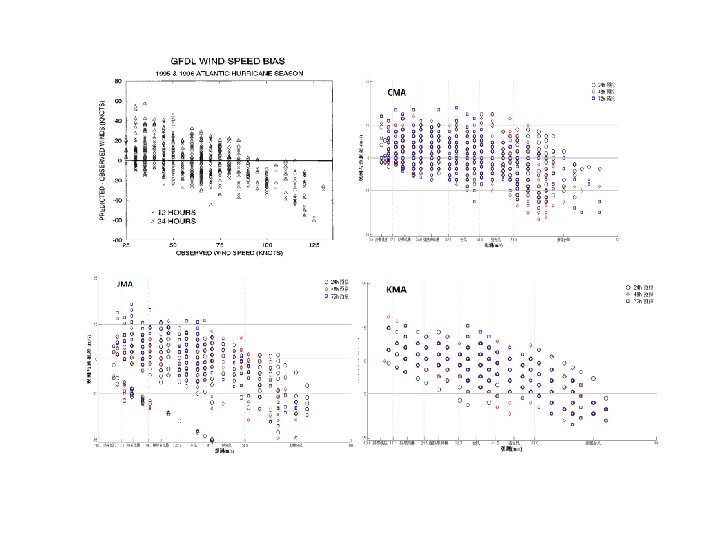
4. Surface wave in Typhoon model

Typhoon/hurricane intensity

Without spray With spray Latent HF Without spray With spray Sensible HF

FIO-AOW ECWMF coupled model Technical Memoranda No. 794 Typhoo n Min/Max MSLP (h. Pa) Haiyan Jebi Max wind(m/s) MSLP (h. Pa) Max wind(m/s) Best track 895 E 0 E 1 E 2 E 123 921. 1 921. 3 892. 7 892. 9 64. 3 58. 0 57. 11 67. 4 66. 7 985 975. 6 977. 9 969. 8 975. 2 25. 7 34. 8 31. 1 40. 1 35. 7 895. 7 68. 7 976. 3 32. 1 Wind-pressure relationship

5. Surface wave in climate system In tropical area, Bv has no much improvements for the ocean circulation model compared with mid- and high latitudes. For full coupled climate model, it is a different story because of the feedback and nonlinearity.

50 a averaged SST (251 -300 a) of CCSM 3. Up: No. Bv-Levitus, Down: Bv-No. Bv Song et al, 2012, JGR

Summertime oceanic mixed layers are biased shallow in both the GFDL and NCAR climate models (Bates et al. 2012; Dunne et al. 2012, 2013). This scheme (Qiao et al. , 2004) has most impact in our simulations on deepening the summertime mixed layers, yet it has minimal impact on wintertime mixed layers. Yalin Fan, and Stephen M. Griffies, 2014, JC (Fig 3)

FIO-ESM for CMIP 5 Wave-induced mixing, Qiao et al. , 2004 Land carbon CASA’ Ocean carbon OCMIP-2 Atmosphere CO 2 transport Framework of FIO-ESM version 1. 0

SST absolute mean errors for 45 CMIP 5 models

Sea ice annual cycle in Arctic

Centurial Future Projections RCP 85 RCP 60 RCP 45 RCP 26 Historical run 3. 9℃

Time series of Arctic sea ice extent from RCP run. Unit: m 2

Component FIO-ESM 2 ATM LND OCN ICE FIO-ESM v 1 FIO-ESM v 2 Model CAM 3 CAM 4, CAM 5 Resolution H: 300 km; V: 26 level H: 200, 100 and 50 km; V: 26 level Model CLM 3. 5 CLM 4. 5 Resolution 300 km 200, 100, and 50 km Model POP 2 NEMO 3. 6 Resolution H: 100 km; V: 40 level; C: 24 hrs H: 100, 50, and 25 km; V: 75 level; C: 24 hrs, 3 hrs Model CICE 4 CICE 5 Resolution 100 km 100, 50, and 25 km Model MASNUM Resolution 200 km 200, 100, and 50 41 km WAV

6. Discussion and suggestions

(1) Compare the results with 107 buoys during 2014 -2015 TAO: Tep Profile 23； 20℃Depth 67；Current 16 RAMA: Tep Profile 23； 20℃Depth 6；Current 22 PIRATA: Tep Profile 17； 20℃Depth 4； Current 1

Temperature profiles of 23 TAO buoys FIOCOM HYCOM Mean Error -0. 028 -0. 051 AME 0. 468 0. 493 RMS 0. 577 0. 620

20 ℃Iosbath of 67 TAO buoys FIOCOM HYCOM Mean Error 0. 60 -0. 05 AME 7. 91 8. 13 RMS 9. 66 10. 27

Current at 16 TAO buoy stations (29 layers) FIOCOM HYCOM Mean Error -1. 93 -12. 03 AME 18. 25 37. 51 RMS 22. 62 44. 62

(2) Data assimilation for climate model

RMS errors with and without DA in climate model 1. 2 1. 0 0. 8 0. 6 0. 4 0. 2 0. 0 6. 0 5. 0 4. 0 3. 0 2. 0 1. 0 0. 0 16. 0 14. 0 12. 0 10. 0 8. 0 6. 0 4. 0 2. 0 0. 0 海表温度/℃ 垂直�速 /10 -3 Pa*s-1 60% 50% 2. 0 10. 0 8. 0 6. 0 4. 0 2. 0 0. 0 1. 5 1. 0 0. 5 0. 0 1. 8 1. 6 1. 4 1. 2 1. 0 0. 8 0. 6 0. 4 0. 2 0. 0 比湿/10 -2 g*kg-1 降水/mm*day-1 35% 37% 3. 5 3. 0 2. 5 2. 0 1. 5 1. 0 0. 5 0. 0 7. 0 6. 0 5. 0 4. 0 3. 0 2. 0 1. 0 0. 0 水平�速 /m*s-1 �云量 /% 上�海洋�含量 /1019 J 海平面气� /h. Pa 26% 25% 21% 19%

Suggestions on pilot projects of TPOS 2020 p Modeling and data assimilation weather to seasonal prediction; from p Pilot observation activities in the tropical oceans from FIO; p The ocean satellite implementation plan till 2025 both in China and other countries.

Thanks for your attention