Tirgul 13 Dast 2010 Union Find DFS Topological

Tirgul 13 - Dast 2010. Union Find – DFS, Topological Sort and SCC School of Computer Science and Engineering, The Hebrew University of Jerusalem. 01: 20: 11 1

Union Find – An Data Structure for Disjoint Sets (Partition) 01: 20: 11 2

A Data Structure for Disjoint Sets • Collection of disjoint sets • makeset(x): create a singleton set containing just x. • find(x): to which set does x belong? «Test pairs of objects to see if they belong to the same set. «Returns a representative of the set. • union(x, y): merge the sets containing x and y. 01: 20: 11 3

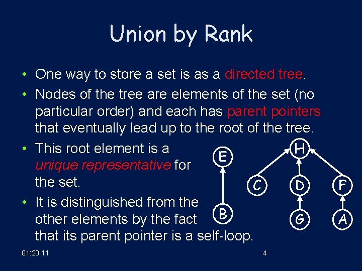
Union by Rank • One way to store a set is as a directed tree. • Nodes of the tree are elements of the set (no particular order) and each has parent pointers that eventually lead up to the root of the tree. • This root element is a H E unique representative for the set. C D • It is distinguished from the B other elements by the fact G that its parent pointer is a self-loop. 01: 20: 11 4 F A

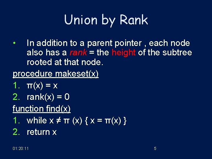
Union by Rank • In addition to a parent pointer , each node also has a rank = the height of the subtree rooted at that node. procedure makeset(x) 1. π(x) = x 2. rank(x) = 0 function find(x) 1. while x ≠ π (x) { x = π(x) } 2. return x 01: 20: 11 5

Union by Rank • makeset is a constant-time operation. • find follows parent pointers to the root of the tree → time proportional to the height of the tree. • The tree actually gets built via union, and so we want union to keep trees shallow. • Merging two sets is easy: make the root of one point to the root of the other. If the representatives (roots) of the sets are rx and ry, do we make rx point to ry 01: 20: 12 6 or the other way around?

Union by Rank • Since tree height is the main limitation to computational efficiency, a good strategy is to make the root of the shorter tree point to the root of the taller tree. • This way, the overall height increases only if the two trees being merged are equally tall. • Instead of explicitly computing heights of trees, we will use the rank numbers of their root nodes. 01: 20: 12 7

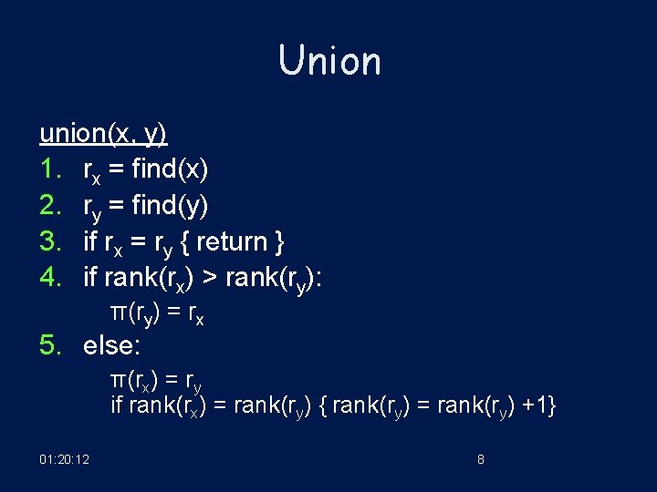
Union union(x, y) 1. rx = find(x) 2. ry = find(y) 3. if rx = ry { return } 4. if rank(rx) > rank(ry): π(ry) = rx 5. else: π(rx) = ry if rank(rx) = rank(ry) { rank(ry) = rank(ry) +1} 01: 20: 12 8

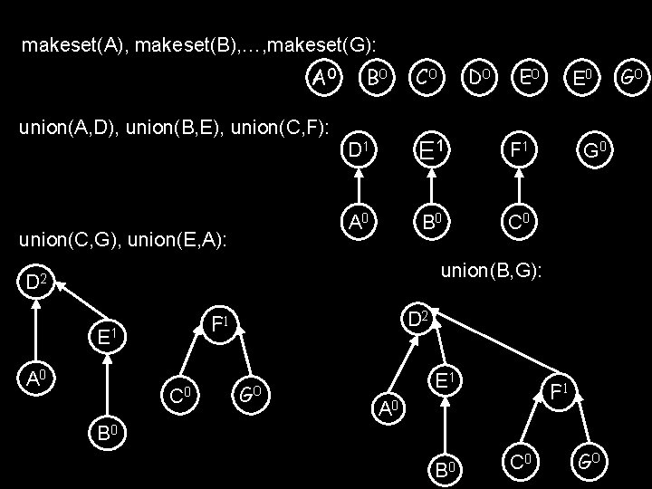
makeset(A), makeset(B), …, makeset(G): A 0 B 0 union(A, D), union(B, E), union(C, F): union(C, G), union(E, A): C 0 D 0 E 0 D 1 E 1 F 1 A 0 B 0 C 0 E 0 G 0 union(B, G): D 2 E 1 A 0 D 2 F 1 C 0 G 0 E 1 F 1 A 0 B 0 C 0 G 0

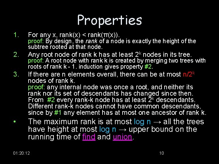
Properties 1. For any x, rank(x) < rank(π(x)). 2. Any root node of rank k has at least 2 k nodes in its tree. 3. If there are n elements overall, there can be at most n/2 k nodes of rank k. proof: any internal node was once a root, and neither its rank nor its set of descendants has changed since then. From #2 every rank-k node has at least 2 k descendants. Different rank-k nodes cannot have common descendants, since by #1 any element has at most one ancestor of rank k. • The maximum rank is at most log n → all the trees have height at most log n → upper bound on the running time of find and union. proof: By design, the rank of a node is exactly the height of the subtree rooted at that node. proof: A root node with rank k is created by merging two trees with roots of rank k - 1. induction gives property #2. 01: 20: 12 10

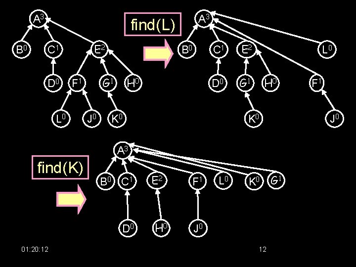
Path compression • Can we improve the performance beyond log n? • Extra effort put into routine maintenance can pay off in the long run. • Our maintenance operation is intended to keep the trees short. • During each find, when a series of parent pointers is followed up to the root of a tree, we will change all these pointers so that they point directly to the root. • This path compression heuristic only slightly increases the time needed for a find. 01: 20: 12 11

A 3 B 0 A 3 find(L) E 2 C 1 D 0 G 1 F 1 L 0 B 0 J 0 H 0 C 1 E 2 D 0 G 1 K 0 L 0 H 0 K 0 J 0 A 3 find(K) B 0 C 1 D 0 01: 20: 12 E 2 H 0 F 1 L 0 K 0 J 0 12 F 1 G 1

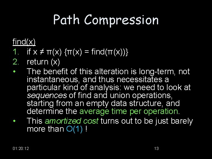
Path Compression find(x) 1. if x ≠ π(x) {π(x) = find(π(x))} 2. return (x) • The benefit of this alteration is long-term, not instantaneous, and thus necessitates a particular kind of analysis: we need to look at sequences of find and union operations, starting from an empty data structure, and determine the average time per operation. • This amortized cost turns out to be just barely more than O(1) ! 01: 20: 12 13

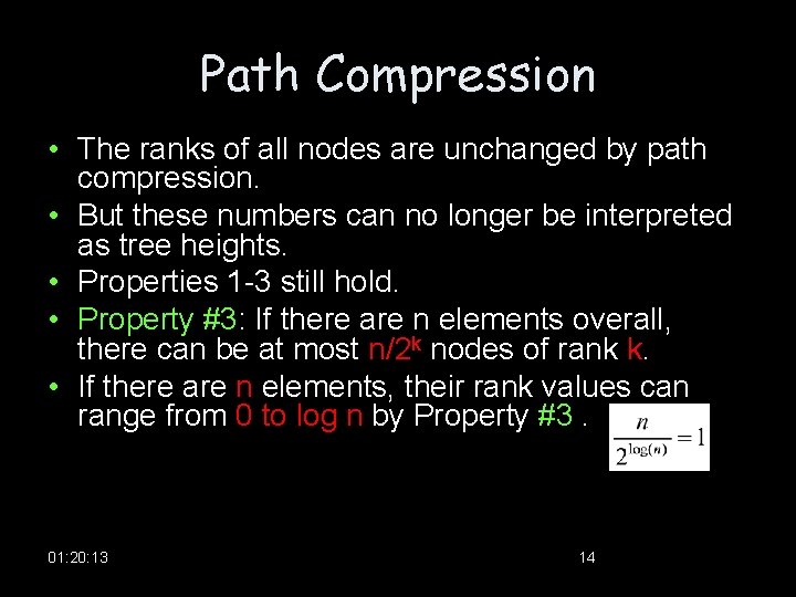
Path Compression • The ranks of all nodes are unchanged by path compression. • But these numbers can no longer be interpreted as tree heights. • Properties 1 -3 still hold. • Property #3: If there are n elements overall, there can be at most n/2 k nodes of rank k. • If there are n elements, their rank values can range from 0 to log n by Property #3. 01: 20: 13 14

Path Compression • In order to calculate the amortized cost we would like to calculate the overall time of m find/union operation. • Since a union operation does 2 find operations and some constant number of O(1) operation, we can limit the analysis to m find operation. • Before we start the analysis we need some preliminaries. 01: 20: 14 15

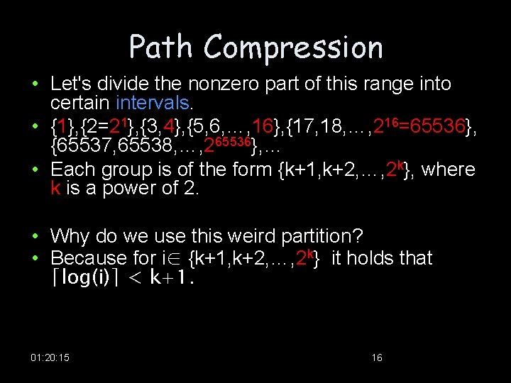
Path Compression • Let's divide the nonzero part of this range into certain intervals. • {1}, {2=21}, {3, 4}, {5, 6, …, 16}, {17, 18, …, 216=65536}, {65537, 65538, …, 265536}, … • Each group is of the form {k+1, k+2, …, 2 k}, where k is a power of 2. • Why do we use this weird partition? • Because for i∈ {k+1, k+2, …, 2 k} it holds that ⌈log(i)⌉ < k+1. 01: 20: 15 16

Path Compression • The number of groups is thus log*n, which is defined to be the number of successive log operations that need to be applied to n to bring it down to 1 (or below 1). • For instance, log*1000=4, since : log log 1000 ≤ 1. • In practice, there will just be the first five of the intervals shown; more are needed only if n ≥ 265536, in other words never. 01: 20: 15 17

Creative Accounting • We will give each node a certain amount of pocket money/time, such that the total money we spend is at most n log*n dollars. • We will then show that each find takes O(log*n) steps, plus some additional amount of time that can be “paid for” using the pocket money of the nodes involved-one dollar per unit of time. • Thus the overall time for m find's is O(mlog*n) plus at most O(nlog*n). 01: 20: 15 18

How Much Money We Give the Nodes ? • A node receives its allowance as soon as it ceases to be a root, at which point its rank is fixed. If this rank lies in the interval {k+1, …, 2 k}, the node receives 2 k dollars. • By Property #3, the number of nodes with rank > k is bounded by: n/2 k+1 + n/2 k+2 +…≤n/2 k • Therefore, the total money given to nodes in this particular interval is at most n dollars, and since there are log*n intervals, the total money disbursed to all nodes is ≤ n log*n. 01: 20: 15 19

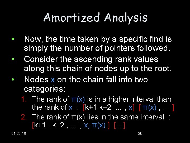
Amortized Analysis • • • Now, the time taken by a specific find is simply the number of pointers followed. Consider the ascending rank values along this chain of nodes up to the root. Nodes x on the chain fall into two categories: 1. The rank of π(x) is in a higher interval than the rank of x : [k+1, k+2, … , x] [ π(x) , … ] 2. The rank of π(x) lies in the same interval : [k+1 , k+2 , … , x, π(x) ] […] 01: 20: 16 20

Amortized Analysis • There at most log*n nodes of the first type, because there are log*n groups. • So the work done on them takes O(log*n) time (we pay). • The remaining nodes-whose parents' ranks are in the same interval as theirshave to pay a dollar out of their pocket money for their processing time. 01: 20: 16 21

Creative Accounting • This only works if the initial allowance of each node x is enough to cover all of its payments in the sequence of m find operations. • Here's the crucial observation: each time x pays a dollar, its parent changes to one of higher rank. Therefore, if x's rank lies in the interval {k+1, …, 2 k}, it has to pay at most 2 k dollars before its parent's rank is in a higher interval; whereupon it never has to pay again. 01: 20: 16 22

Explore – DFS –Topological Sort – SCC 01: 20: 16 23

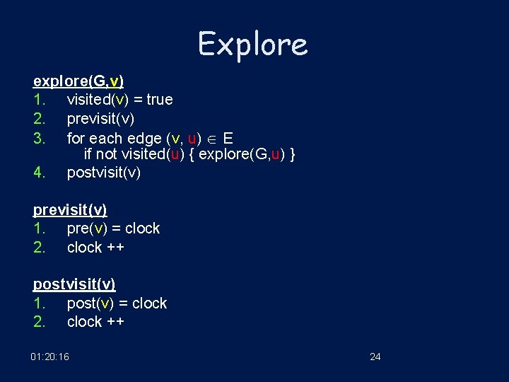
Explore explore(G, v) 1. visited(v) = true 2. previsit(v) 3. for each edge (v, u) E if not visited(u) { explore(G, u) } 4. postvisit(v) previsit(v) 1. pre(v) = clock 2. clock ++ postvisit(v) 1. post(v) = clock 2. clock ++ 01: 20: 16 24

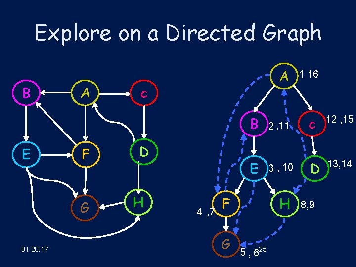
Explore on a Directed Graph B E A F G 01: 20: 17 A c D H 4 , 7 B E F G 2 , 11 c 12 , 15 3 , 10 D 13, 14 H 5 , 625 1 16 8, 9

DFS • The explore procedure visits only parts of the graph reachable from its starting point. • To examine the rest of the graph, we need to restart the procedure elsewhere, at some node that has not yet been visited. • The algorithm depth-first search (DFS), does this repeatedly until the entire graph has been traversed. • DFS calls explore to vertices which were not visited yet. 01: 20: 17 26

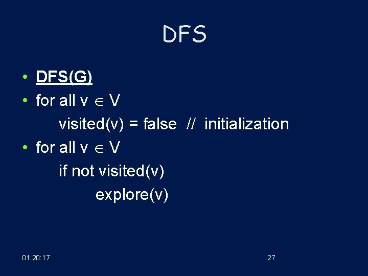
DFS • DFS(G) • for all v V visited(v) = false // initialization • for all v V if not visited(v) explore(v) 01: 20: 17 27

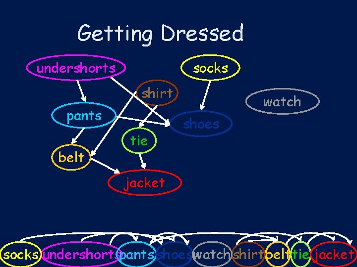
Getting Dressed undershorts socks shirt pants belt tie watch shoes jacket socks undershortspants shoes watch shirt belt tie jacket

Topological Sort • What types of DAGs can be linearized? • As we have seen in class: All of them. • Explore search tells us exactly how to do it: simply perform tasks in decreasing order of their post numbers. • Property: In a DAG, every edge leads to a node with a lower post number. 01: 20: 17 29

Topological Sort –Algorithm • This gives a linear-time algorithm for ordering the nodes of a DAG: topological sort(G) 1. DFS(G) 2. Sort the nodes by decreasing post numbers. • When DFS departures the t node, we can store it in index n-t in an output array. • Time complexity: O(|E|+|V|) (DFS) 01: 20: 17 30

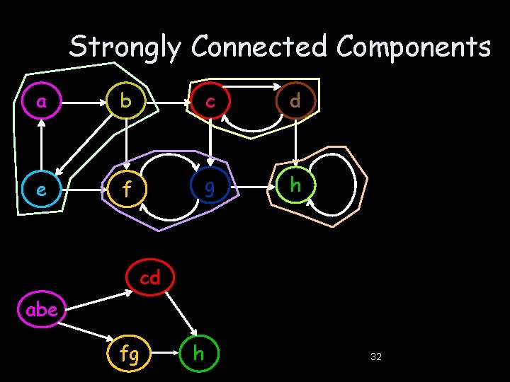
Strongly Connected Components • A strongly connected component C ⊆ V is a maximal set such that for every u, v ∈ C there is a paths u⇝v and a path v⇝u. • Every graph can be partitioned in to strongly connected components. • If each strongly connected component is contracted to a single vertex, the resulting graph is a DAG (why? ), and is called the strongly connected components graph. 01: 20: 17 31

Strongly Connected Components a b c d e f g h cd abe fg h 32

Strongly Connected Components • As we have seen in class a property very similar to what we seen in topologic sorts holds for SCCs: • Property 1: If there exists an edge from a SCC C 1 to another SCC C 2 then the maximal post time of a vertex in C 1 is larger then the maximal post time of a vertex in C 2 (why? ). • Property 2: The set of SCCs of GR is equal to the set of SCC of G. 01: 20: 18 33

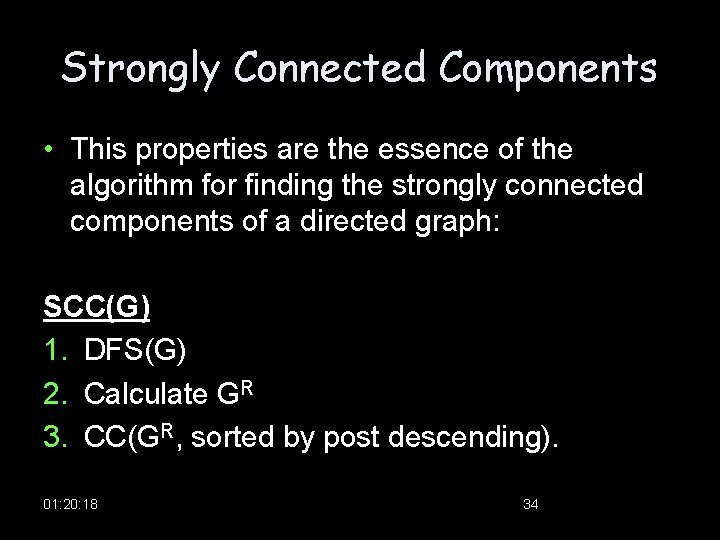
Strongly Connected Components • This properties are the essence of the algorithm for finding the strongly connected components of a directed graph: SCC(G) 1. DFS(G) 2. Calculate GR 3. CC(GR, sorted by post descending). 01: 20: 18 34

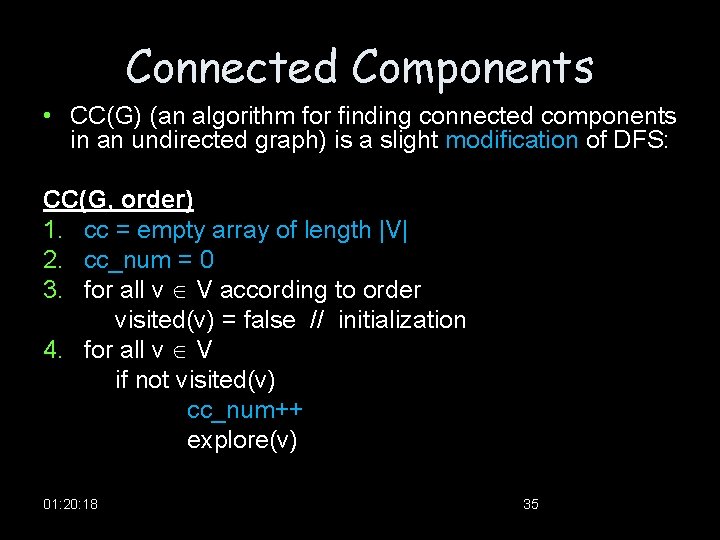
Connected Components • CC(G) (an algorithm for finding connected components in an undirected graph) is a slight modification of DFS: CC(G, order) 1. cc = empty array of length |V| 2. cc_num = 0 3. for all v V according to order visited(v) = false // initialization 4. for all v V if not visited(v) cc_num++ explore(v) 01: 20: 18 35

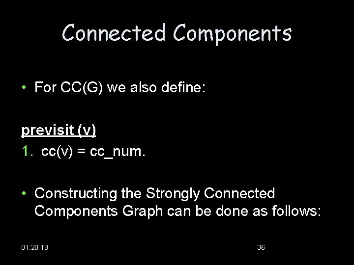
Connected Components • For CC(G) we also define: previsit (v) 1. cc(v) = cc_num. • Constructing the Strongly Connected Components Graph can be done as follows: 01: 20: 18 36

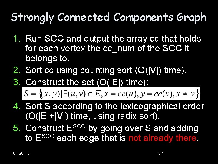
Strongly Connected Components Graph 1. Run SCC and output the array cc that holds for each vertex the cc_num of the SCC it belongs to. 2. Sort cc using counting sort (O(|V|) time). 3. Construct the set (O(|E|) time): 4. Sort S according to the lexicographical order (O(|E|+|V|) time, using radix sort). 5. Construct ESCC by going over S and adding to ESCC each edge that is not already there. 01: 20: 18 37

Strongly Connected Components Graph • #5 can be done efficiently since S is already sorted. Just delete all but one consecutive identical entries: for i=1 to |S| if S(i) == S(i+1) then remove S(i+1) • The total worst case running time of the algorithm is O(|V|+|E|). 01: 20: 18 38