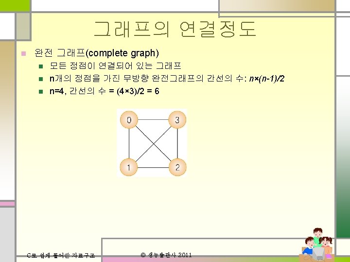
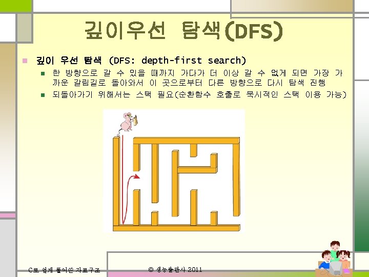
n DFS BFS n n DFS BFS visitedvTRUE

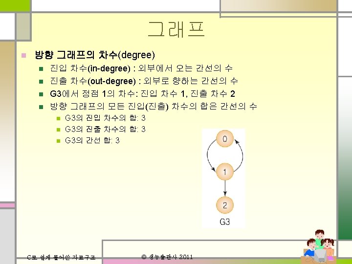


연결 성분 최대로 연결된 부분 그래프들 n DFS 또는 BFS 반복 이용 n n DFS 또는 BFS 탐색 프로그램의 visited[v]=TRUE; 를 visited[v]=count; 로 교체 int count; void find_connected_component(Graph. Type *g) { int i; count = 0; for(i=0; i<g->n; i++) if(!visited[i]){ // 방문되지 않았으면 count++; dfs_mat(g, i); } } C로 쉽게 풀어쓴 자료구조 © 생능출판사 2011
![union-find 프로그램 int parent[MAX_VERTICES]; int num[MAX_VERTICES]; void set_init(int n) { int i; for(i=0; i<n;](http://slidetodoc.com/presentation_image_h/c5b7d80394957a6bb7059818f9a4ac08/image-34.jpg "union-find 프로그램 int parent[MAX_VERTICES]; int num[MAX_VERTICES]; void set_init(int n) { int i; for(i=0; i<n;")
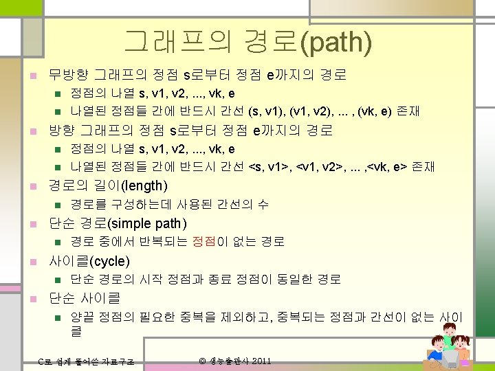
union-find 프로그램 int parent[MAX_VERTICES]; int num[MAX_VERTICES]; void set_init(int n) { int i; for(i=0; i<n; i++){ parent[i] = -1; num[i] = 1; } } // 부모 노드 // 각 집합의 크기 // 초기화 vertex 0 1 2 3 4 5 6 parent[] -1 -1 num[] 1 1 1 1 set_union(1, 4) set_union(5, 2) int set_find(int vertex) // vertex가 속하는 집합 반환 { int p, s, i=-1; vertex for(i=vertex; (p=parent[i])>=0; i=p) ; // 루트 노드까지 반복 parent[] s = i; // 집합의 대표 원소 num[] for(i=vertex; (p=parent[i])>=0; i=p) parent[i] = s; // 집합의 모든 원소들의 부모를 s로 설정 return s; } void set_union(int s 1, int s 2) { if( num[s 1] < num[s 2] ){ parent[s 1] = s 2; num[s 2] += num[s 1]; } else { parent[s 2] = s 1; num[s 1] += num[s 2]; } } C로 쉽게 풀어쓴 자료구조 // 두 개의 원소가 속한 집합을 합함 0 1 2 3 4 5 6 -1 -1 5 -1 1 -1 -1 1 2 1 set_union(4, 5) [set_find(4); set_union(1, 5)] set_union(3, 6) vertex 0 1 2 3 4 5 6 parent[] -1 -1 5 -1 1 1 3 num[] 1 4 1 2 1 © 생능출판사 2011

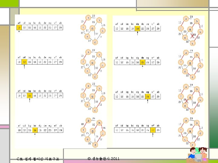
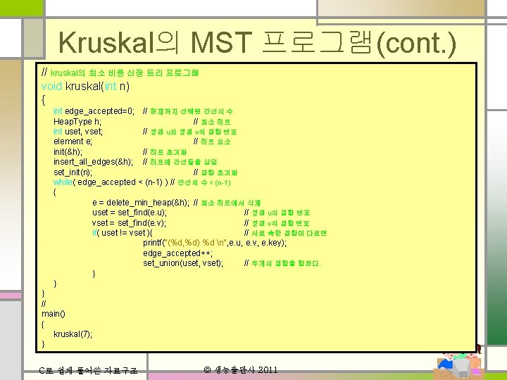
Kruskal의 MST 프로그램 #include <stdio. h> #define MAX_VERTICES 100 #define INF 1000 // 프로그램 10. 7의 union-find 프로그램 삽입 //. . . // 히프의 요소 타입 정의 typedef struct { int key; // 간선의 가중치 int u; // 정점 1 int v; // 정점 2 } element; // 프로그램 8. 5 중에서 최소 히프 프로그램 삽입 //. . . // 정점 u와 정점 v를 연결하는 가중치가 weight인 간선을 히프에 삽입 void insert_heap_edge(Heap. Type *h, int u, int v, int weight) { element e; e. u = u; e. v = v; e. key = weight; insert_min_heap(h, e); } // 인접 행렬이나 인접 리스트에서 간선들을 읽어서 최소 히프에 삽입 // 현재는 예제 그래프의 간선들을 삽입한다. void insert_all_edges(Heap. Type *h){ insert_heap_edge(h, 0, 1, 29); insert_heap_edge(h, 1, 2, 16); insert_heap_edge(h, 2, 3, 12); insert_heap_edge(h, 3, 4, 22); insert_heap_edge(h, 4, 5, 27); insert_heap_edge(h, 5, 0, 10); insert_heap_edge(h, 6, 1, 15); insert_heap_edge(h, 6, 3, 18); insert_heap_edge(h, 6, 4, 25); } © 생능출판사 2011 C로 쉽게 풀어쓴 자료구조
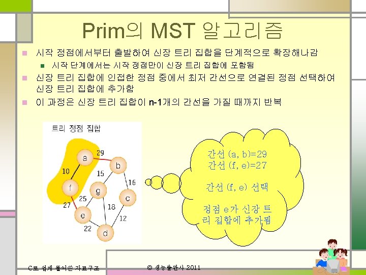
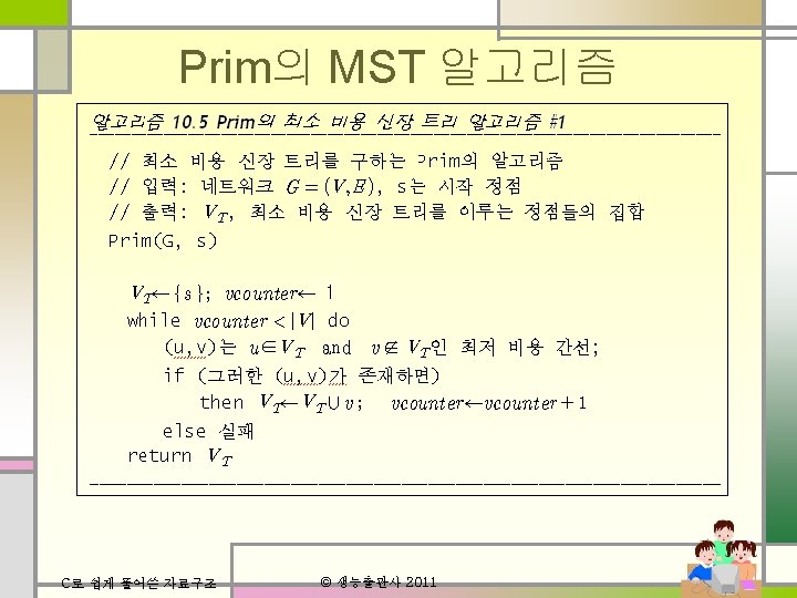
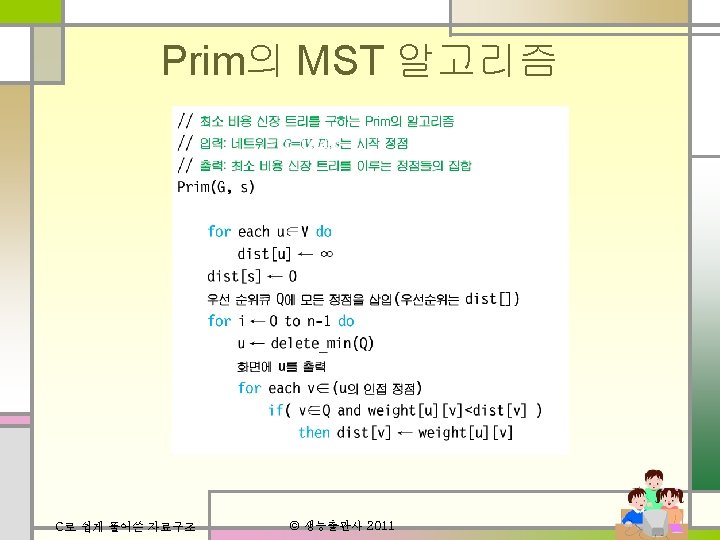

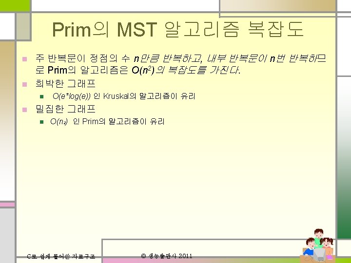
Prim의 MST 프로그램 #include <stdio. h> #define TRUE 1 #define FALSE 0 #define MAX_VERTICES 7 #define INF 1000 L int weight[MAX_VERTICES]={ { 0, 29, INF, 10, INF }, { 29, 0, 16, INF, 15 }, { INF, 16, 0, 12, INF, INF }, { INF, 12, 0, 22, INF, 18 }, { INF, 22, 0, 27, 25 }, { 10, INF, 27, 0, INF }, { INF, 15, INF, 18, 25, INF, 0 }}; int selected[MAX_VERTICES]; int dist[MAX_VERTICES]; // 최소 dist[v] 값을 갖는 정점을 반환 int get_min_vertex(int n) { int v, i; for (i = 0; i <n; i++) if (!selected[i]) { v = i; break; } for (i = 0; i < n; i++) if ( !selected[i] && (dist[i] < dist[v])) v = i; return (v); } 쉽게 풀어쓴 자료구조 © 생능출판사 2011 C로
 void prim(int s, int n) { int i, u, v;")
Prim의 MST 프로그램(cont. ) void prim(int s, int n) { int i, u, v; for(u=0; u<n; u++) dist[u]=INF; dist[s]=0; for(i=0; i<n; i++){ u = get_min_vertex(n); selected[u]=TRUE; if( dist[u] == INF ) return; printf("%d ", u); for( v=0; v<n; v++) if( weight[u][v]!= INF) if( !selected[v] && weight[u][v]< dist[v] ) dist[v] = weight[u][v]; } } // main() { prim(0, MAX_VERTICES); } C로 쉽게 풀어쓴 자료구조 © 생능출판사 2011
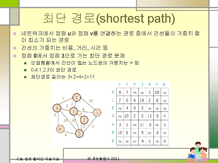

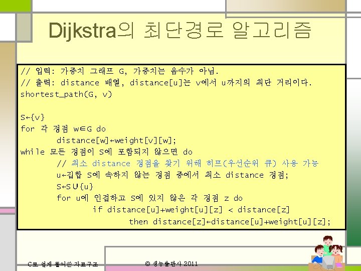
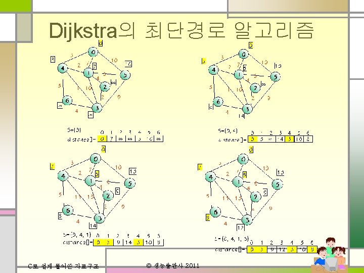
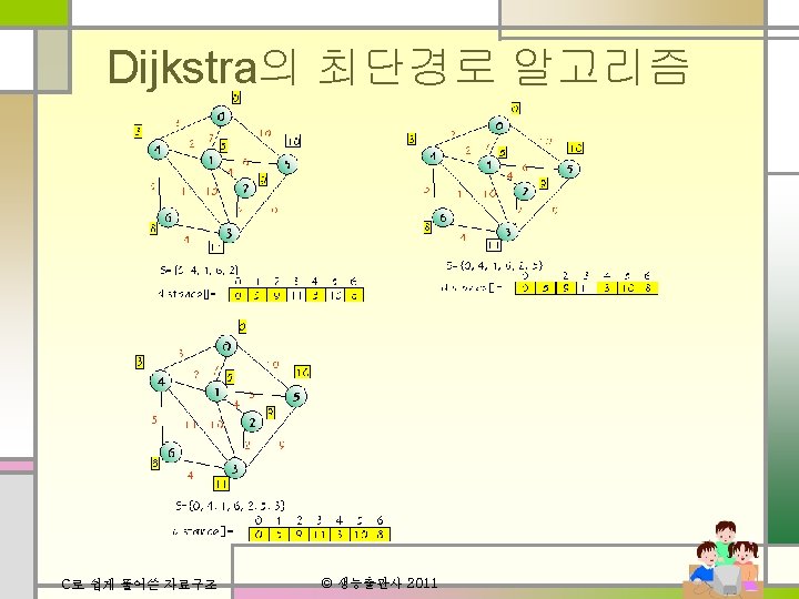

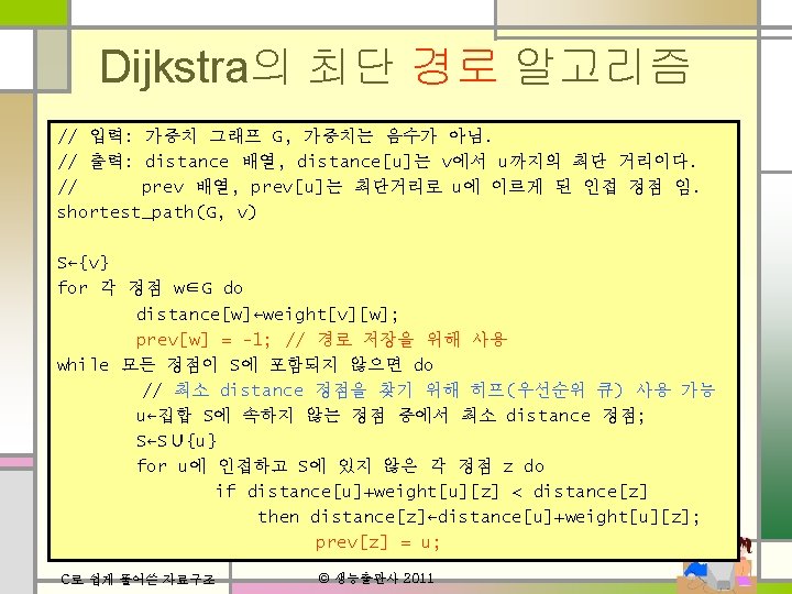
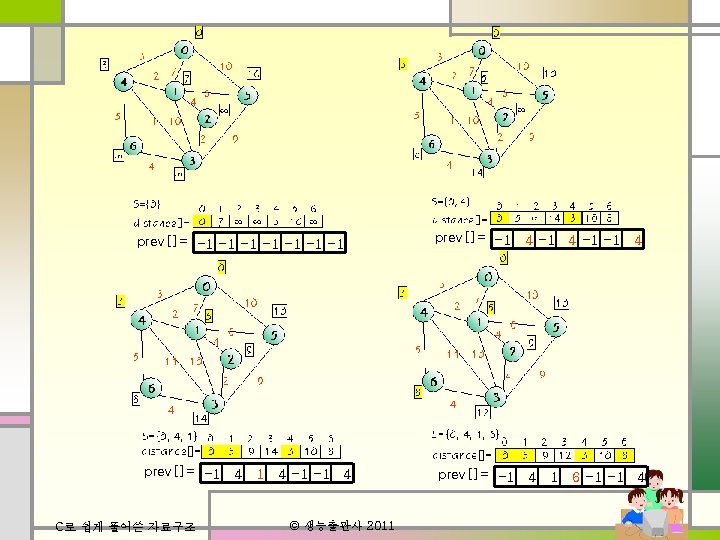
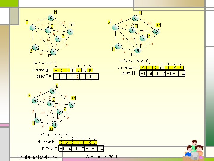
Dijkstra의 최단경로 프로그램 #include <stdio. h> #include <limits. h> #define TRUE 1 #define FALSE 0 #define MAX_VERTICES 7 // 정점의 수 #define INF 1000 // 무한대 (연결이 없는 경우) int weight[MAX_VERTICES]={ // 네트워크의 인접 행렬 { 0, 7, INF, 3, 10, INF }, { 7, 0, 4, 10, 2, 6, INF }, { INF, 4, 0, 2, INF, INF }, { INF, 10, 2, 0, 11, 9, 4 }, { 3, 2, INF, 11, 0, INF, 5 }, { 10, 6, INF, 9, INF, 0, INF }, { INF, 4, 5, INF, 0 }}; int distance[MAX_VERTICES]; // 시작정점으로부터의 최단경로 거리 int found[MAX_VERTICES]; // 방문한 정점 표시 // int choose(int distance[], int n, int found[]) { int i, minpos; min = INT_MAX; minpos = -1; for(i=0; i<n; i++) if( distance[i]< min && ! found[i] ){ min = distance[i]; minpos=i; } return minpos; } C로 쉽게 풀어쓴 자료구조 © 생능출판사 2011
 void shortest_path(int start, int n) { int i, u, w;")
Dijkstra의 최단경로 프로그램(cont. ) void shortest_path(int start, int n) { int i, u, w; for(i=0; i<n; i++) // 초기화 { distance[i] = weight[start][i]; found[i] = FALSE; } found[start] = TRUE; // 시작 정점 방문 표시 distance[start] = 0; for(i=0; i<n-2; i++){ u = choose(distance, n, found); found[u] = TRUE; for(w=0; w<n; w++) if(!found[w]) if( distance[u]+weight[u][w]<distance[w] ) distance[w] = distance[u]+weight[u][w]; } } // void main() { shortest_path(0, MAX_VERTICES); } 쉽게 풀어쓴 자료구조 © 생능출판사 2011 C로

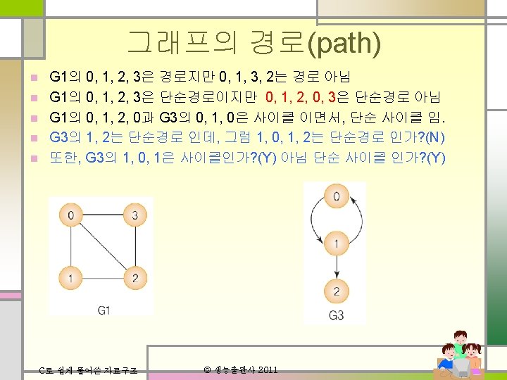
![Floyd의 최단경로 프로그램 int A[MAX_VERTICES]; void floyd(int n) { int i, j, k; for(i=0;](http://slidetodoc.com/presentation_image_h/c5b7d80394957a6bb7059818f9a4ac08/image-60.jpg "Floyd의 최단경로 프로그램 int A[MAX_VERTICES]; void floyd(int n) { int i, j, k; for(i=0;")
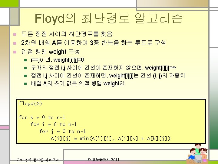
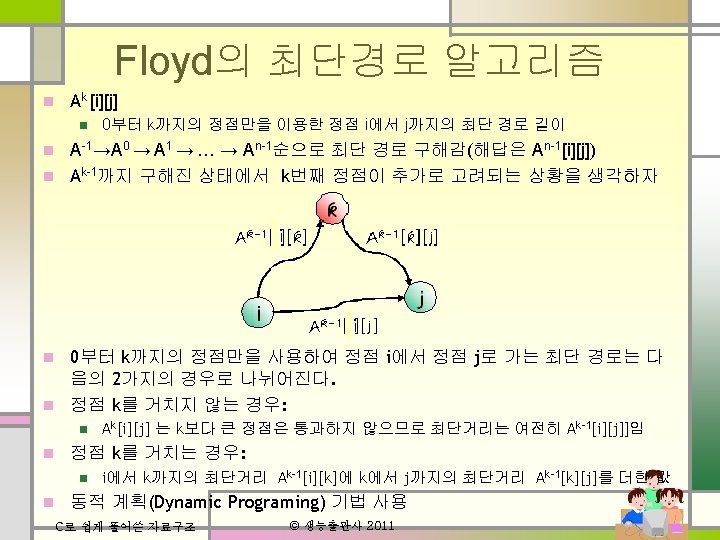
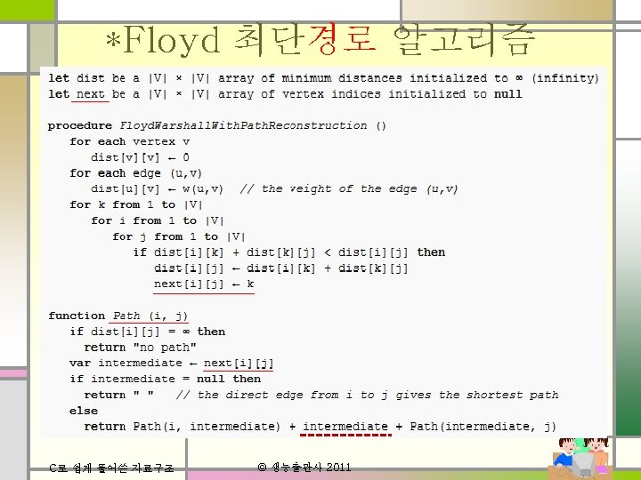
Floyd의 최단경로 프로그램 int A[MAX_VERTICES]; void floyd(int n) { int i, j, k; for(i=0; i<n; i++) for(j=0; j<n; j++) A[i][j]=weight[i][j]; for(k=0; k<n; k++) for(i=0; i<n; i++) for(j=0; j<n; j++) if (A[i][k]+A[k][j] < A[i][j]) A[i][j] = A[i][k]+A[k][j]; } C로 쉽게 풀어쓴 자료구조 © 생능출판사 2011

Floyd 최단경로 알고리즘 예 0 7 7 0 3 10 4 10 2 6 4 0 2 10 2 0 11 9 4 3 2 11 0 13 5 10 6 9 13 0 4 0 A-1 5 A 0 0 7 11 17 3 10 0 7 11 13 3 10 17 7 0 4 10 2 6 7 0 4 6 2 11 4 0 2 6 10 6 17 10 2 0 11 9 4 13 6 2 0 8 9 4 0 8 5 3 2 6 8 0 8 5 6 10 9 8 0 10 6 10 9 8 0 13 4 5 0 17 10 4 5 13 3 10 2 6 11 6 10 9 8 0 10 4 5 0 A 1 C로 쉽게 풀어쓴 자료구조 A 2 © 생능출판사 2011 6 A 3 6 10 0

Floyd 최단경로 알고리즘 예 0 7 11 13 3 10 17 7 0 4 6 2 11 4 0 2 6 10 6 13 6 2 0 8 9 4 3 2 6 8 0 8 5 6 10 9 8 0 13 4 5 13 10 17 10 6 A-1 6 10 0 A 3 0 5 9 11 3 10 8 5 0 4 6 2 6 7 9 4 0 2 6 10 6 11 6 2 0 8 9 4 3 2 6 8 0 8 5 6 10 9 8 0 13 10 6 10 9 8 0 13 7 4 5 13 10 8 6 A 4 C로 쉽게 풀어쓴 자료구조 0 8 6 A 5 © 생능출판사 2011 0 8 6 A 6 0
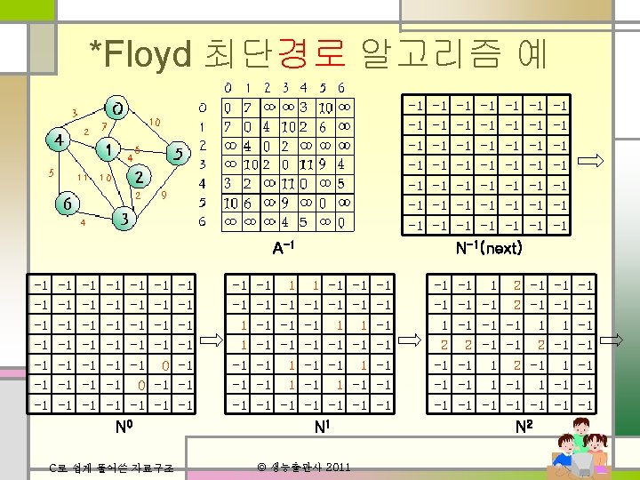

*Floyd 최단경로 알고리즘 예 -1 -1 1 2 -1 -1 -1 1 2 2 -1 -1 1 2 -1 -1 -1 1 -1 -1 -1 A-1 -1 2 -1 1 3 2 -1 -1 4 3 4 -1 -1 2 -1 -1 3 4 -1 -1 -1 1 4 2 -1 -1 1 2 2 -1 -1 1 -1 3 3 2 -1 1 4 1 -1 -1 -1 3 -1 -1 3 3 -1 N 3 C로 쉽게 풀어쓴 자료구조 -1 4 N 2 2 -1 -1 -1 4 4 2 -1 4 4 -1 -1 4 4 4 -1 -1 2 -1 -1 4 3 4 -1 -1 -1 1 4 2 -1 -1 3 -1 -1 N 4 1 3 3 -1 -1 4 2 -1 -1 -1 4 4 2 -1 1 1 -1 3 -1 -1 3 3 3 -1 N 5 , N 6 Path(0, 3) = Path(0, 4) + Path(4, 3) Path(4, 2) + Path(2, 3) © 생능출판사 2011 Path(4, 1) + Path(1, 2)
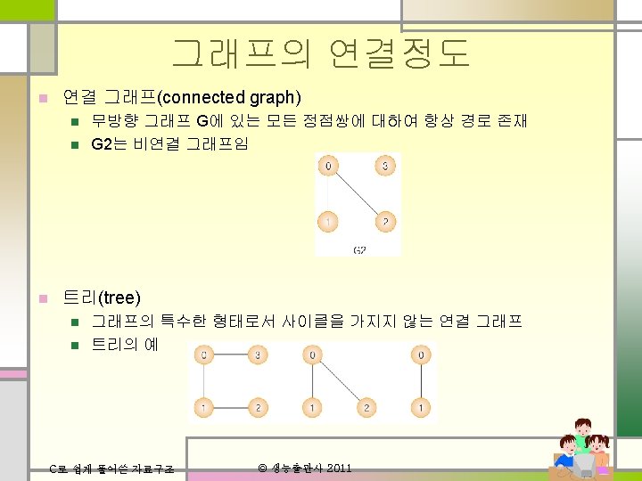
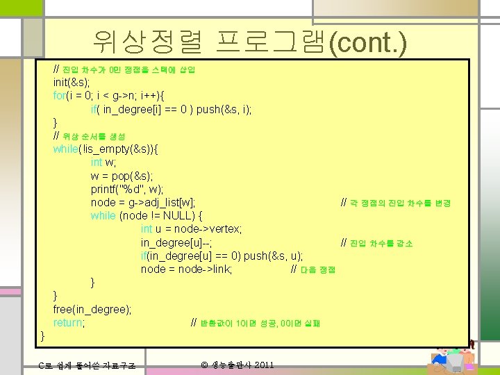
 { int i; Stack. Type s; Graph. Node")
위상정렬 프로그램 void topo_sort(Graph. Type *g) { int i; Stack. Type s; Graph. Node *node; // 모든 정점의 진입 차수를 계산 int *in_degree = (int *)malloc(g->n* sizeof(int)); for(i = 0; i < g->n; i++) // 초기화 in_degree[i] = 0; for(i = 0; i < g->n; i++){ Graph. Node *node = g->adj_list[i]; // 정점 i에서 나오는 간선들 while ( node != NULL ) { in_degree[node->vertex]++; node = node->link; } } C로 쉽게 풀어쓴 자료구조 © 생능출판사 2011
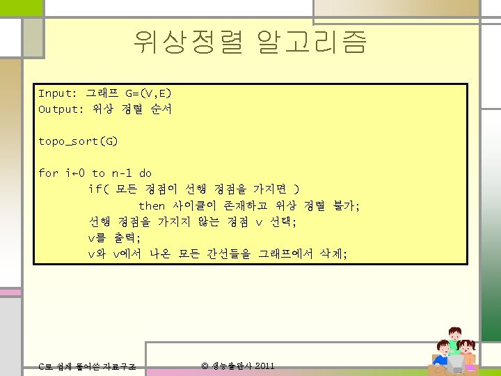
- Slides: 71