Time Series Analysis Chapter 4 Hypothesis Testing Hypothesis

Time Series Analysis – Chapter 4 Hypothesis Testing Hypothesis testing is basic to the scientific method and statistical theory gives us a way of conducting tests of scientific hypotheses. Scientific philosophy today rests on the idea of falsification: For a theory to be a valid scientific theory it must be possible, at least in principle, to make observations that would prove theory false. For example, here is a simple theory: All swans are white

Time Series Analysis – Chapter 4 Hypothesis Testing All swans are white This is a valid scientific theory because there is a way to falsify it: I can observe one black swan and theory would fall. For more information on the history and philosophy of falsification I suggest reading Karl Popper.

Time Series Analysis – Chapter 4 Hypothesis Testing Besides the idea of falsification, we must keep in mind the other basic tenant of the scientific method: All evidence that supports a theory or falsifies it must be empirically based and reproducible.

All evidence that supports a theory or falsifies it must be empirically based and reproducible. In other words, data! Just holding a belief (no matter how firm) that a theory is true or false is not a justifiable stance. This chapter gives us the most basic statistical tools for taking data or empirical evidence and using it to substantiate or nullify (show to be false) a hypothesis.

All evidence that supports a theory or falsifies it must be empirically based and reproducible. I have just used the word hypothesis and this chapter is concerned with hypothesis testing, not theory testing. This is because theories are composed of many hypotheses and, usually, a theory is not directly supported or attacked but one or more of it’s supporting hypotheses are scrutinized.

Discrimination or Not Activity Null Hypothesis Ho: No Discrimination Alternative Hypothesis Ha: Discrimination How do we choose which hypothesis to support?

Discrimination or Not Activity Null Hypothesis Ho: No Discrimination Alternative Hypothesis Ha: Discrimination How do we choose which hypothesis to support?

The p-value • p-value measures amount of support for alternative hypothesis. • The smaller the p-value the more support for the alternative hypothesis. • Typical level of support is 5% or 0. 05

Fourth Graders Feet Data Set

Fourth Graders Feet Data Set – Minitab Output Predictor variable (x): Childs Age Response variable (y): Foot Length The regression equation is Foot Length = 18. 1 + 0. 0358 Childs Age Predictor Coef SE Coef T P Constant 18. 138 3. 753 4. 83 0. 000 Childs Age 0. 03575 0. 02922 1. 22 0. 229

Fourth Graders Feet Data Set – Minitab Output

Fourth Graders Feet Data Set – One Tailed Alternative

Statistical vs. Practical Significance 401 K data set Predictor variables x 1: mrate x 2: age x 3: totemp Response variable (y): prate

Statistical vs. Practical Significance The regression equation is: prate = 80. 3 + 5. 44 mrate + 0. 269 age - 0. 000130 totemp Predictor Coef SE Coef T P Constant 80. 2943 0. 7777 103. 25 0. 000 mrate 5. 4414 0. 5244 10. 38 0. 000 age 0. 26941 0. 04515 5. 97 0. 000 totemp -0. 00012978 0. 00003672 -3. 53 0. 000

Statistical vs. Practical Significance The regression equation is: prate = 80. 3 + 5. 44 mrate + 0. 269 age - 0. 000130 totemp All predictors are statistically significant.

Statistical vs. Practical Significance The regression equation is: prate = 80. 3 + 5. 44 mrate + 0. 269 age - 0. 000130 totemp If total number of employees increases by ten thousand then participation rate decreases by 0. 000130*10, 000 = 1. 3% (other predictors held constant)

Boeing 747 Jet What does an empty Boeing 747 jet weigh?

Boeing 747 Jet What does an empty Boeing 747 jet weigh? My point estimate: 250, 000 lbs Answer: 358, 000 lbs I am wrong! A point estimate is almost always wrong!

Boeing 747 Jet What does an empty Boeing 747 jet weigh? My confidence interval estimate: (0, ∞) Answer: 358, 000 lbs I am right! But, my interval is not useful!

Point and Interval Estimates – Minitab will compute both 401 K data set Predictor variables x 1: age Response variable (y): prate In Minitab go to Regression -> General Regression and select the correct model variables then click on the Results box and make sure the “Display confidence intervals” box is selected.

Point and Interval Estimates – Minitab will compute both 401 K data set Predictor variables x 1: age Response variable (y): prate Regression Equation prate = 83. 4231 + 0. 298893 age Coefficients Term Coef SE Coef T P 95% CI Constant 83. 4231 0. 737593 113. 102 0. 000 (81. 9763, 84. 8699) age 0. 2989 0. 045938 6. 506 0. 000 ( 0. 2088, 0. 3890)

Confidence Intervals

Confidence Intervals

Confidence Intervals

Confidence Intervals Where does 1. 960 come from? t distribution with n – k – 1 degrees of freedom where k is the number of predictors in the model. For our model, n = 1533 and k = 1 We also need to know the confidence level of the interval (typically 95%) Then, use a t table!

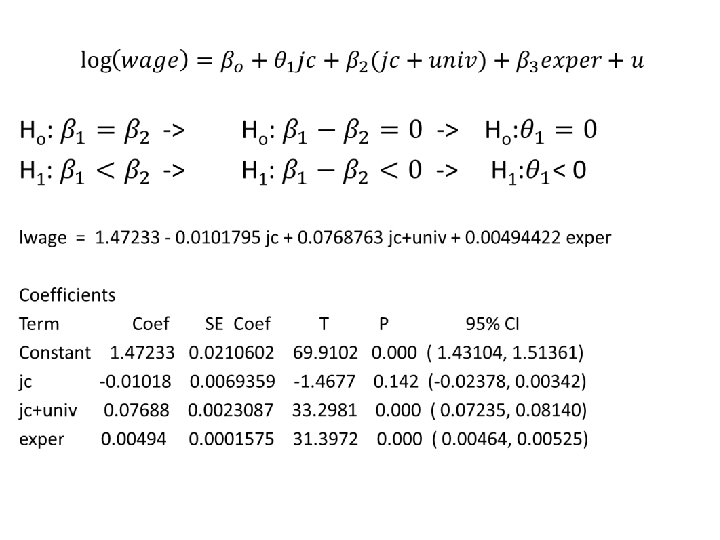
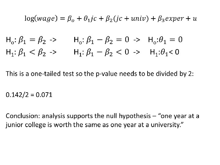
Testing Linear Combinations of Parameters TWOYEAR data set Predictor variables x 1: jc – # years attending a two-year college x 2: univ – # years attending a four-year college x 3: exper – months in workforce Response variable (y): log(wage)

Testing Linear Combinations of Parameters

Testing Linear Combinations of Parameters

Testing Linear Combinations of Parameters

Testing Linear Combinations of Parameters

Testing Linear Combinations of Parameters

Testing Linear Combinations of Parameters

The ANOVA F Test

Multiple Linear Regression Assumptions

Multiple Linear Regression Assumptions MLR Assumption 2: Data comes from a random sample

Multiple Linear Regression Assumptions MLR Assumption 3: None of the independent or predictor variables are perfectly correlated (if they were, Minitab would not run a regression analysis).

Multiple Linear Regression Assumptions MLR Assumption 4: The error, u, has an expected value of zero.

Multiple Linear Regression Assumptions MLR Assumption 5: The error, u, has the same variance given any values of the explanatory variables. This is the assumption of homoskedasticity.

Multiple Linear Regression Assumptions