The Gradient Descent Algorithm Initialize all weights to

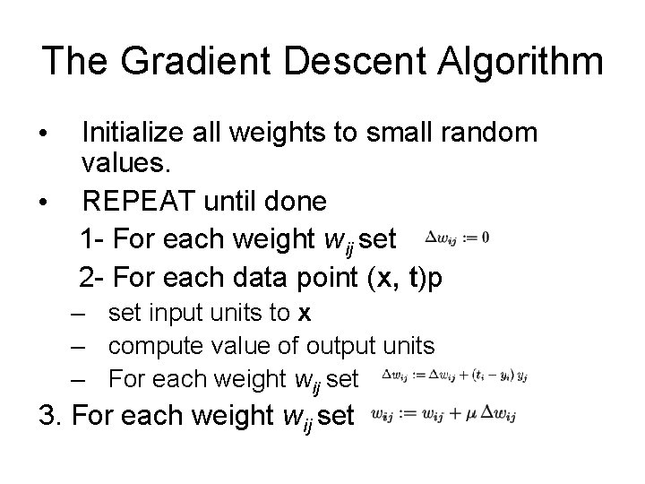
The Gradient Descent Algorithm • • Initialize all weights to small random values. REPEAT until done 1 - For each weight wij set 2 - For each data point (x, t)p – set input units to x – compute value of output units – For each weight wij set 3. For each weight wij set

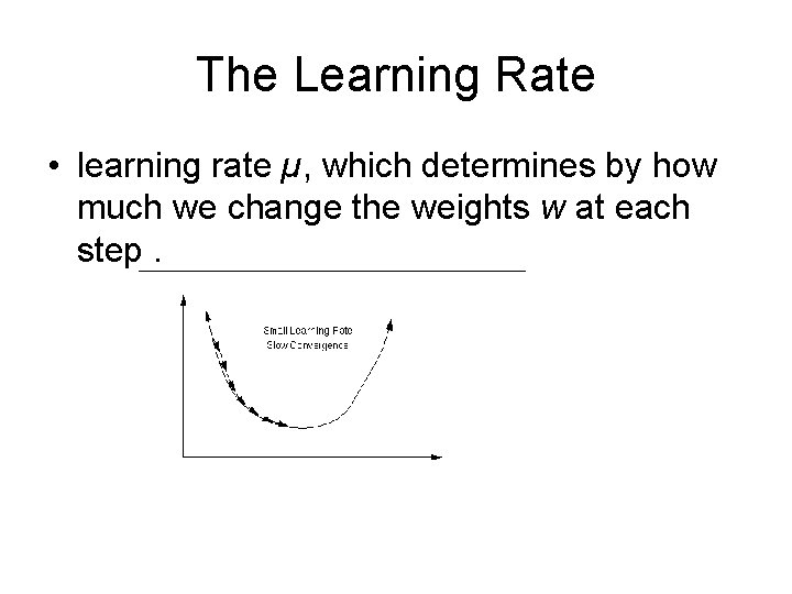
The Learning Rate • learning rate µ, which determines by how much we change the weights w at each step.

Batch vs. Online Learning • The gradient contributions for all data points in the training set are accumulated before updating the weights. This method is often referred to as batch learning. An alternative approach is online learning, where the weights are updated immediately after seeing each data point. Since the gradient for a single data point can be considered a noisy approximation to the overall gradient G (Fig. 5), this is also called stochastic (noisy) gradient descent.

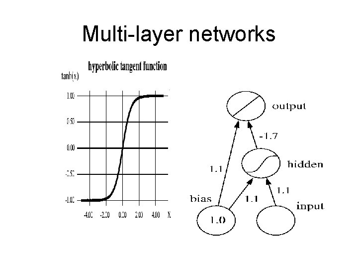
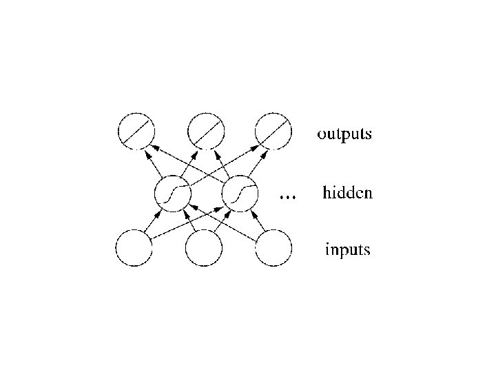
Multi-layer networks

• Too large hidden layer - or too many hidden layers - can degrade the network's performance. • One shouldn't use more hidden units than necessary • Start training with a very small network. • If gradient descent fails to find a satisfactory solution, grow the network by adding a hidden unit, and repeat. • Any function can be expressed as a linear combination of tanh functions: tanh is a universal basis function. • Two classes of activation functions commonly used in neural networks are the sigmoidal (S-shaped) basis functions (to which tanh belongs), and the radial basis functions.

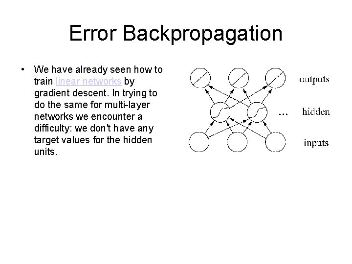
Error Backpropagation • We have already seen how to train linear networks by gradient descent. In trying to do the same for multi-layer networks we encounter a difficulty: we don't have any target values for the hidden units.

The Algorithm • How to train a multi-layer feedforward network by gradient descent to approximate an unknown function, based on some training data consisting of pairs (x, t)?

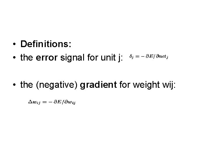
• Definitions: • the error signal for unit j: • the (negative) gradient for weight wij:

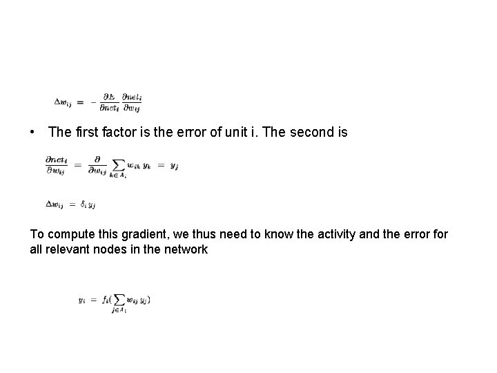
• The first factor is the error of unit i. The second is To compute this gradient, we thus need to know the activity and the error for all relevant nodes in the network

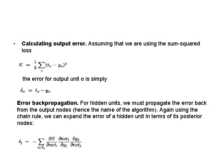
• Calculating output error. Assuming that we are using the sum-squared loss the error for output unit o is simply Error backpropagation. For hidden units, we must propagate the error back from the output nodes (hence the name of the algorithm). Again using the chain rule, we can expand the error of a hidden unit in terms of its posterior nodes:

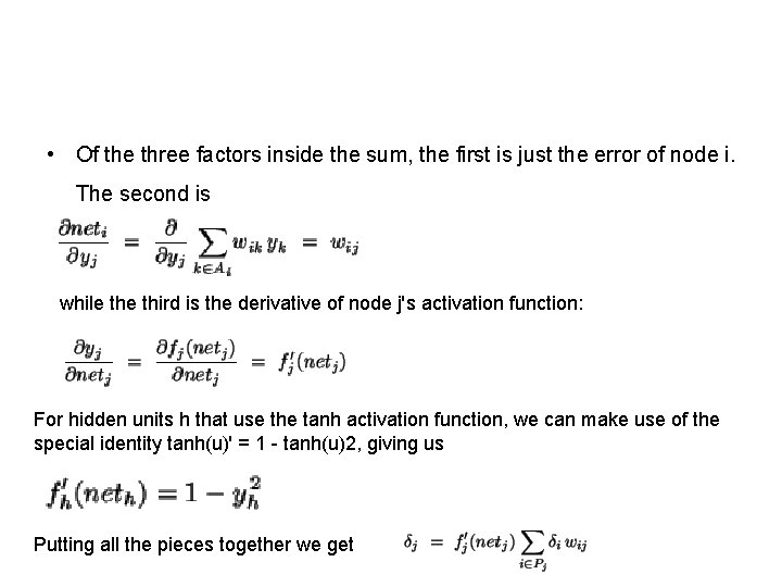
• Of the three factors inside the sum, the first is just the error of node i. The second is while third is the derivative of node j's activation function: For hidden units h that use the tanh activation function, we can make use of the special identity tanh(u)' = 1 - tanh(u)2, giving us Putting all the pieces together we get

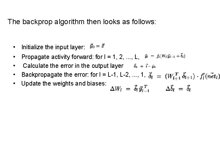
The backprop algorithm then looks as follows: • Initialize the input layer: • Propagate activity forward: for l = 1, 2, . . . , L, • Calculate the error in the output layer • Backpropagate the error: for l = L-1, L-2, . . . , 1, • Update the weights and biases:

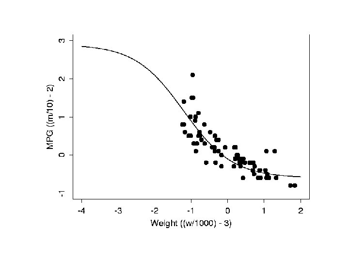
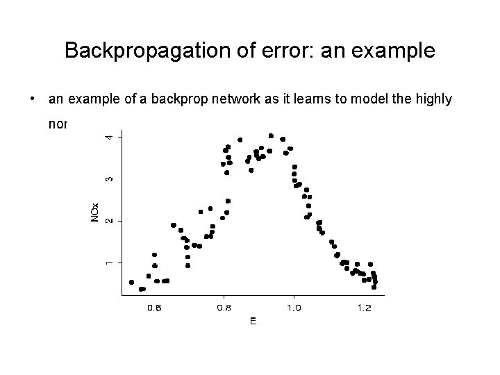
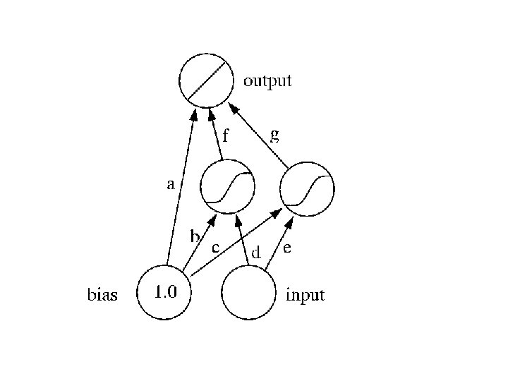
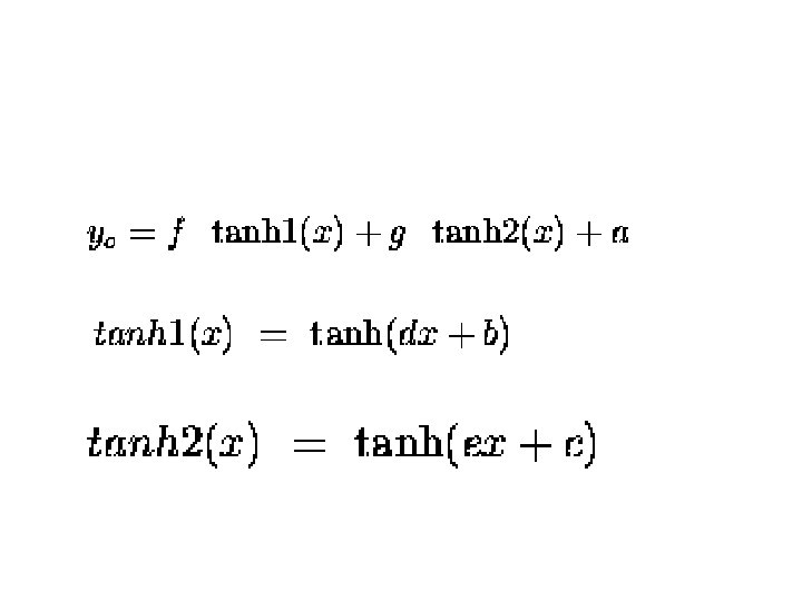
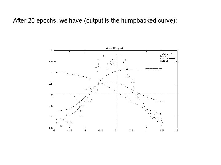
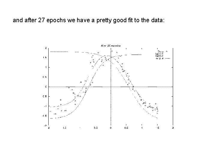
Backpropagation of error: an example • an example of a backprop network as it learns to model the highly nonlinear data

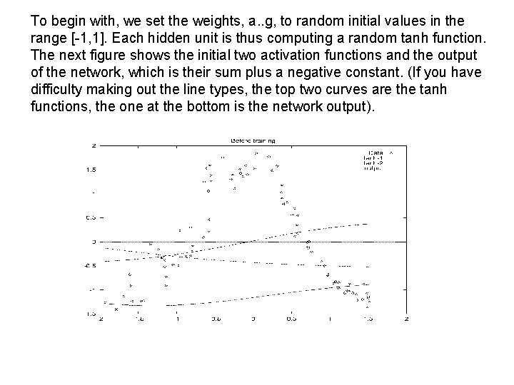
To begin with, we set the weights, a. . g, to random initial values in the range [-1, 1]. Each hidden unit is thus computing a random tanh function. The next figure shows the initial two activation functions and the output of the network, which is their sum plus a negative constant. (If you have difficulty making out the line types, the top two curves are the tanh functions, the one at the bottom is the network output).

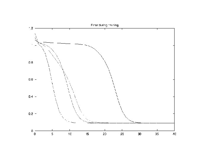
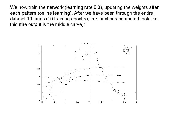
We now train the network (learning rate 0. 3), updating the weights after each pattern (online learning). After we have been through the entire dataset 10 times (10 training epochs), the functions computed look like this (the output is the middle curve):

After 20 epochs, we have (output is the humpbacked curve):

and after 27 epochs we have a pretty good fit to the data: