Gradient Methods Steepest Descent gradient descent Conjugate Gradient

Gradient Methods: Steepest Descent (gradient descent), Conjugate Gradient.

Problem: finding local minimum.

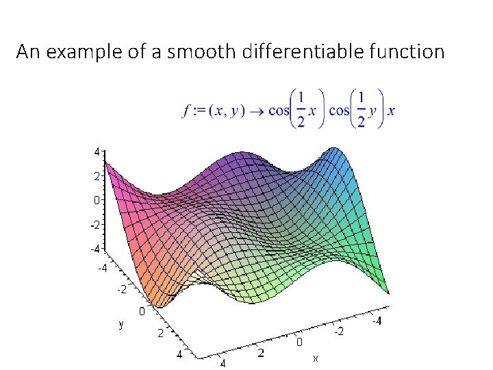
An example of a smooth differentiable function

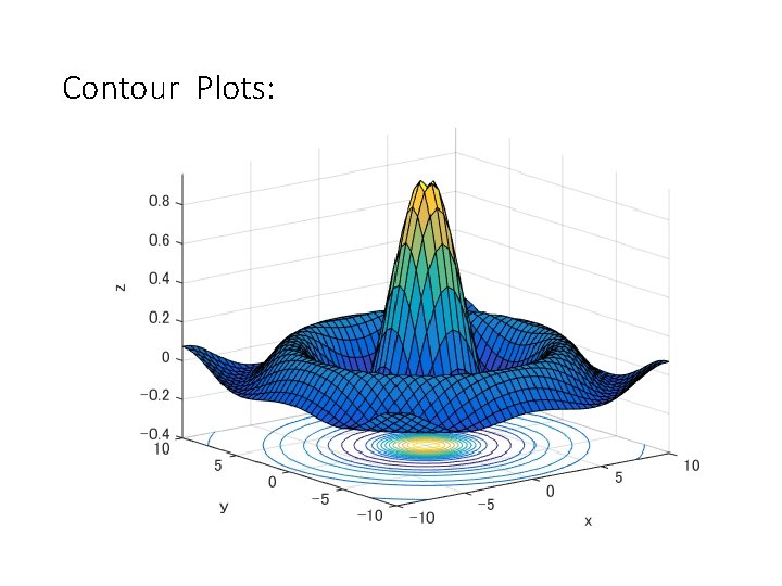
Contour Plots:

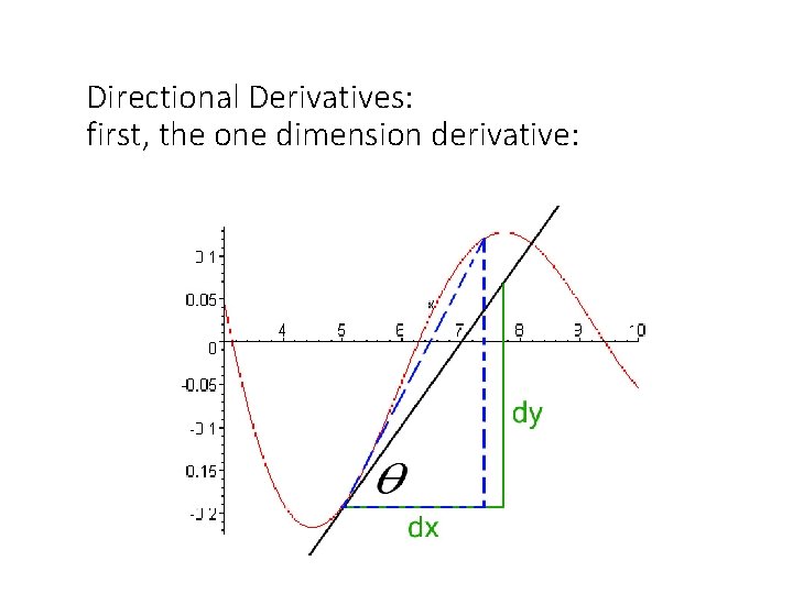
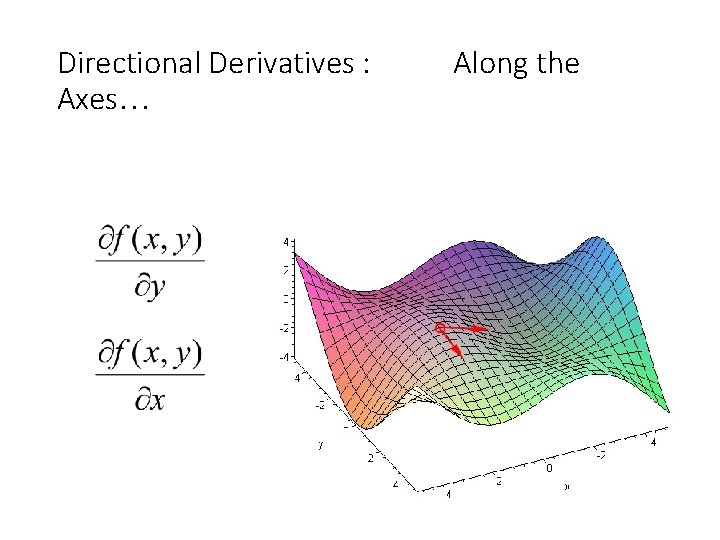
Directional Derivatives: first, the one dimension derivative:

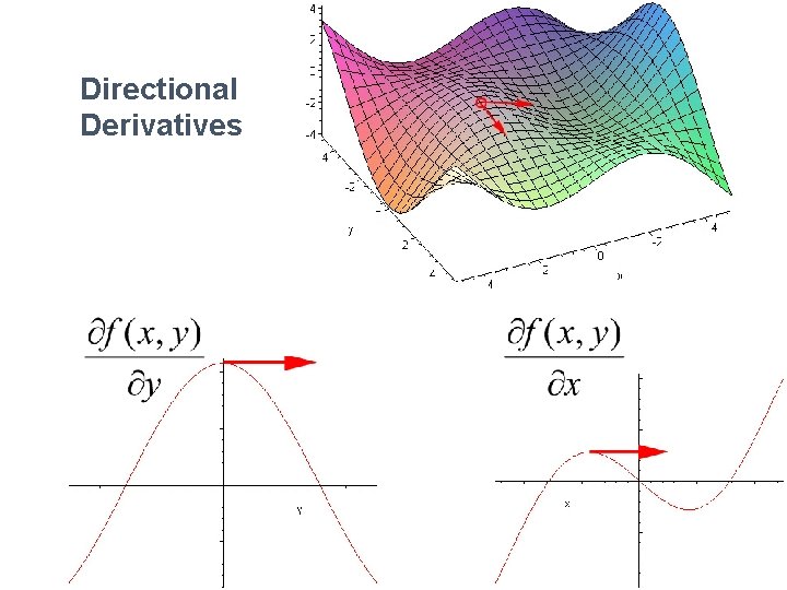
Directional Derivatives : Axes… Along the

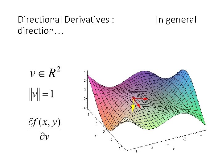
Directional Derivatives : direction… In general

Directional Derivatives

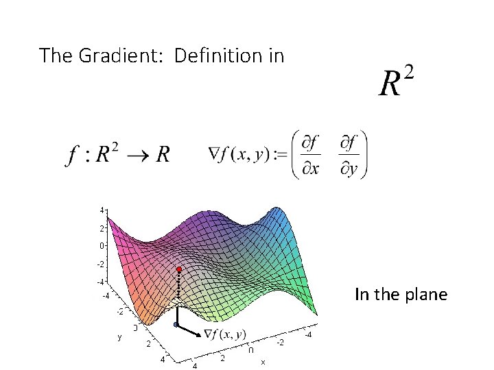
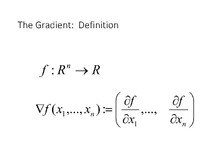
The Gradient: Definition in In the plane

The Gradient: Definition

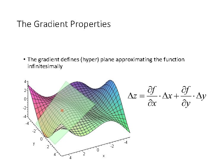
The Gradient Properties • The gradient defines (hyper) plane approximating the function infinitesimally

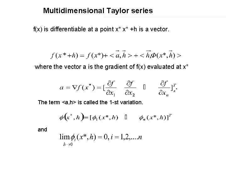
Multidimensional Taylor series f(x) is differentiable at a point x* x* +h is a vector. where the vector a is the gradient of f(x) evaluated at x* The term <a, h> is called the 1 -st variation. and

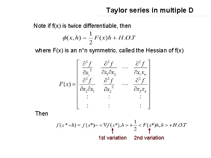
Taylor series in multiple D Note if f(x) is twice differentiable, then where F(x) is an n*n symmetric, called the Hessian of f(x) Then 1 st variation 2 nd variation

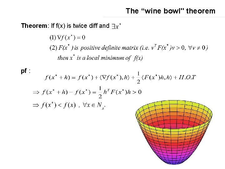
The “wine bowl" theorem Theorem: If f(x) is twice diff and pf :

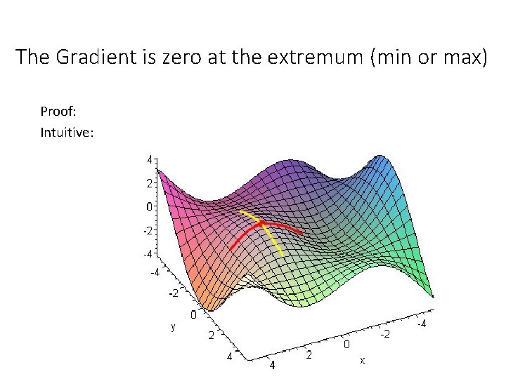
The Gradient is zero at the extremum (min or max) Proof: Intuitive:

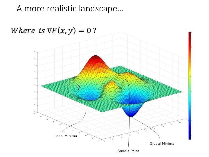
A more realistic landscape…

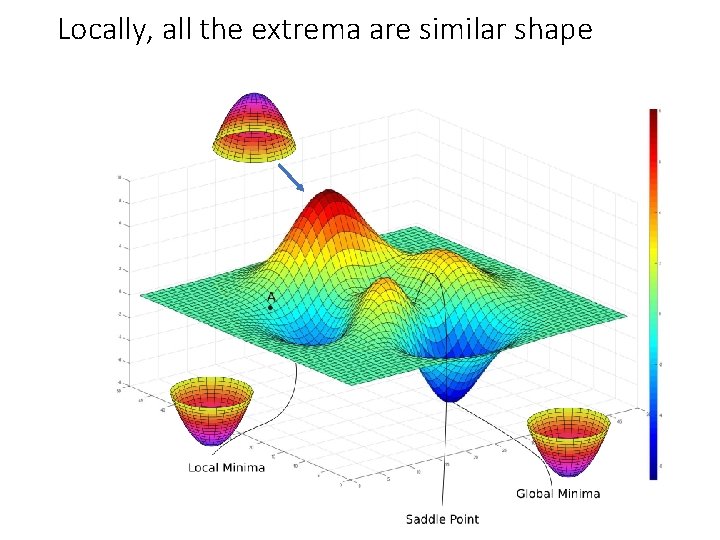
Locally, all the extrema are similar shape

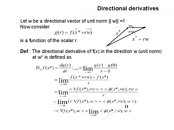
Directional derivatives Let w be a directional vector of unit norm || w|| =1 Now consider is a function of the scalar r. Def : The directional derivative of f(x) in the direction w (unit norm) at w* is defined as

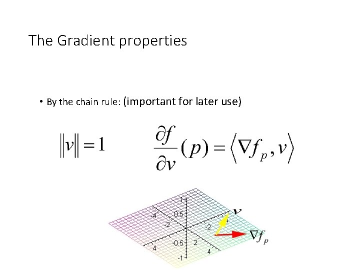
The Gradient properties • By the chain rule: (important for later use)

Unconstrained Minimization [Q] : What direction w yield the largest directional derivative? Ans : [A]: The direction of the gradient is the direction that yields the largest change (1 st -variation) in the function. This suggests the steepest decent method:

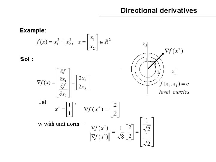
Directional derivatives Example: Sol : Let , w with unit norm =

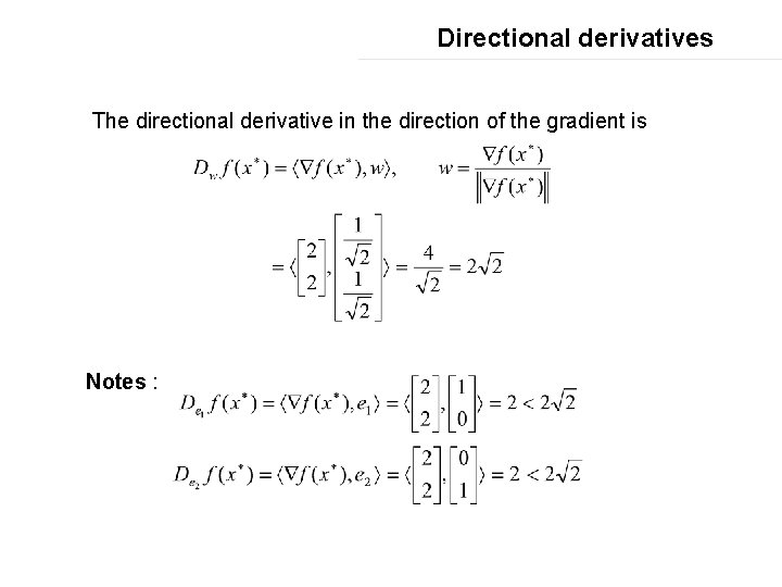
Directional derivatives The directional derivative in the direction of the gradient is Notes :

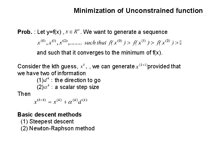
Minimization of Unconstrained function Prob. : Let y=f(x) , . We want to generate a sequence and such that it converges to the minimum of f(x). Consider the kth guess, , we can generate we have two of information (1) the direction to go (2) a scalar step size Then Basic descent methods (1) Steepest descent (2) Newton-Raphson method provided that

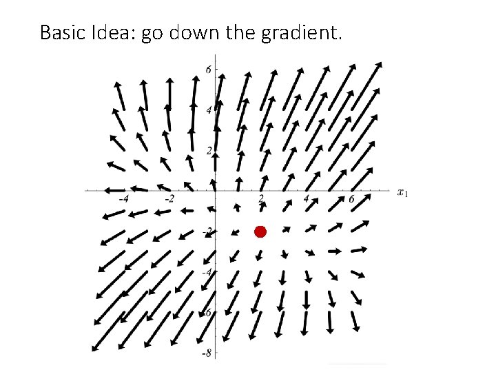
Basic Idea: go down the gradient.

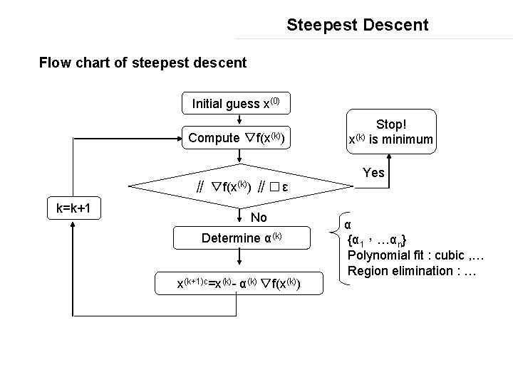
Steepest Descent Flow chart of steepest descent Initial guess x(0) Compute ∥ k=k+1 ▽f(x(k)) ∥� ε No Determine α(k) x(k+1)c=x(k)- α(k) ▽f(x(k)) Stop! x(k) is minimum Yes α {α 1，…αn} Polynomial fit : cubic , … Region elimination : …

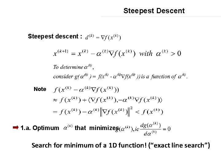
Steepest Descent Steepest descent : Note 1. a. Optimum that minimizes Search for minimum of a 1 D function! (“exact line search”)

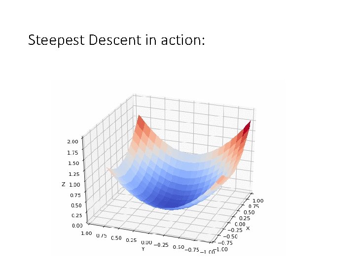
Steepest Descent in action:

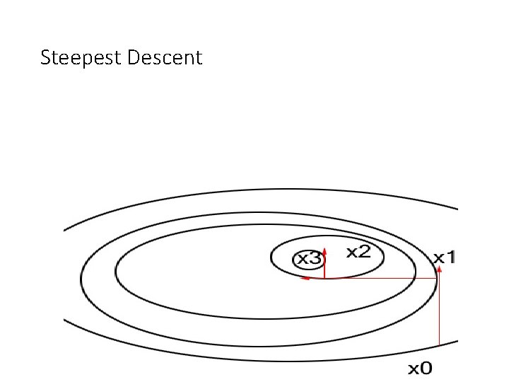
Steepest Descent

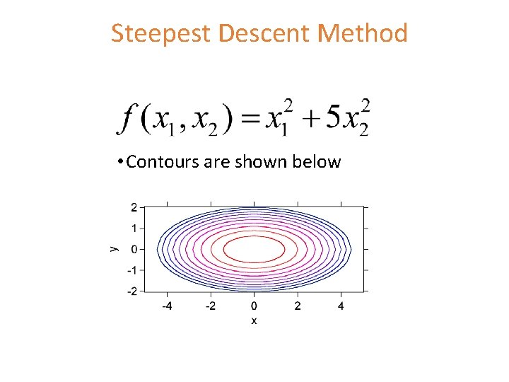
Steepest Descent Method • Contours are shown below

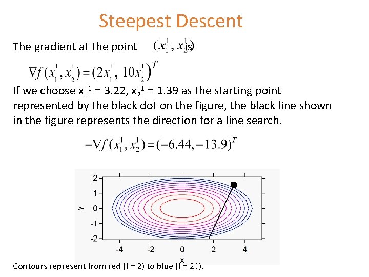
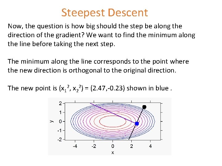
Steepest Descent The gradient at the point is If we choose x 11 = 3. 22, x 21 = 1. 39 as the starting point represented by the black dot on the figure, the black line shown in the figure represents the direction for a line search. Contours represent from red (f = 2) to blue (f = 20).

Steepest Descent Now, the question is how big should the step be along the direction of the gradient? We want to find the minimum along the line before taking the next step. The minimum along the line corresponds to the point where the new direction is orthogonal to the original direction. The new point is (x 12, x 22) = (2. 47, -0. 23) shown in blue.

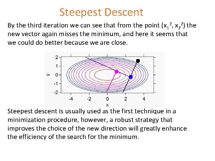
Steepest Descent By the third iteration we can see that from the point (x 12, x 22) the new vector again misses the minimum, and here it seems that we could do better because we are close. Steepest descent is usually used as the first technique in a minimization procedure, however, a robust strategy that improves the choice of the new direction will greatly enhance the efficiency of the search for the minimum.

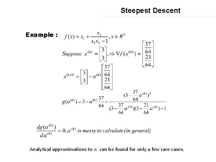
Steepest Descent Example : Analytical approximations to a can be found for only a few rare cases.

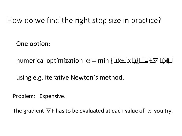
How do we find the right step size in practice? One option: numerical optimization a = min {�� (x+ a�� )}, �� =−∇�� (x) using e. g. iterative Newton’s method. Problem: Expensive. The gradient ∇F has to be evaluated at each value of a you try.

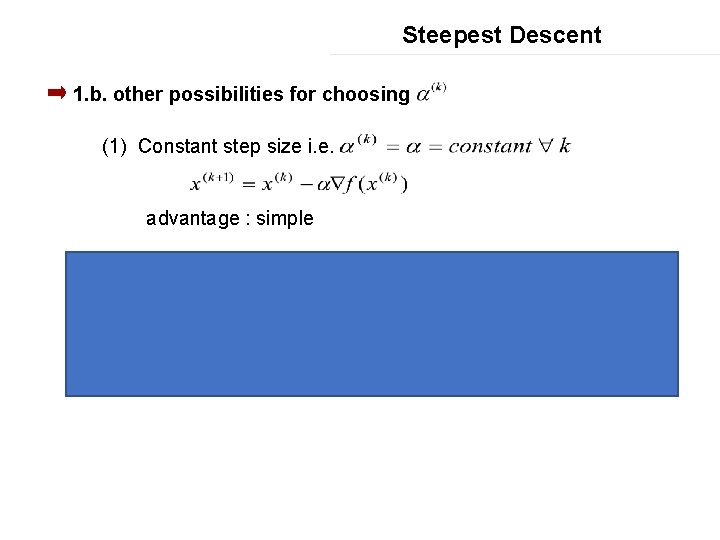
Steepest Descent 1. b. other possibilities for choosing (1) Constant step size i. e. advantage : simple disadvantages : no idea of which value of α to choose If α is too large diverge If α is too small very slow (2) Variable step size

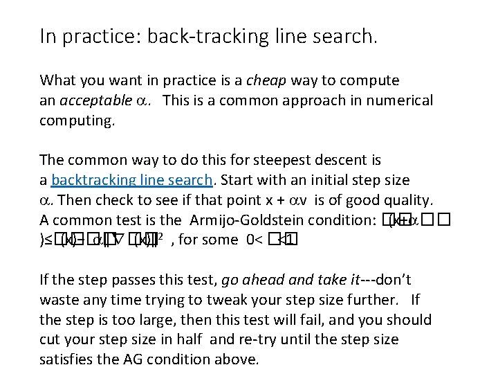
In practice: back-tracking line search. What you want in practice is a cheap way to compute an acceptable a. This is a common approach in numerical computing. The common way to do this for steepest descent is a backtracking line search. Start with an initial step size a. Then check to see if that point x + av is of good quality. A common test is the Armijo-Goldstein condition: �� (x+a�� )≤�� (x)−�� a‖∇�� (x)‖ 2 , for some 0< �� <1. If the step passes this test, go ahead and take it---don’t waste any time trying to tweak your step size further. If the step is too large, then this test will fail, and you should cut your step size in half and re-try until the step size satisfies the AG condition above.

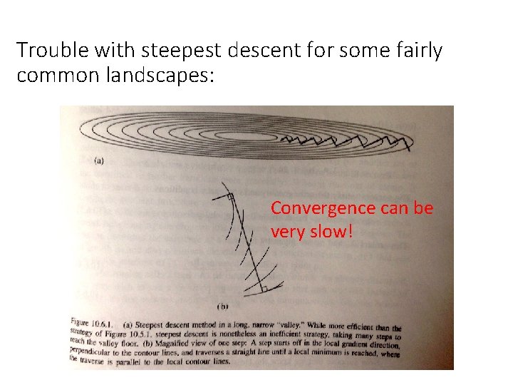
Trouble with steepest descent for some fairly common landscapes: Convergence can be very slow!

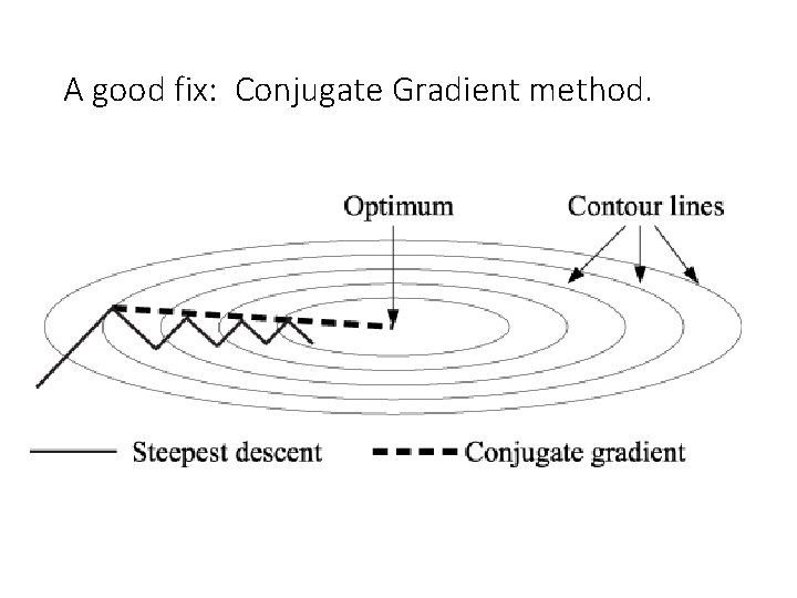
A good fix: Conjugate Gradient method.

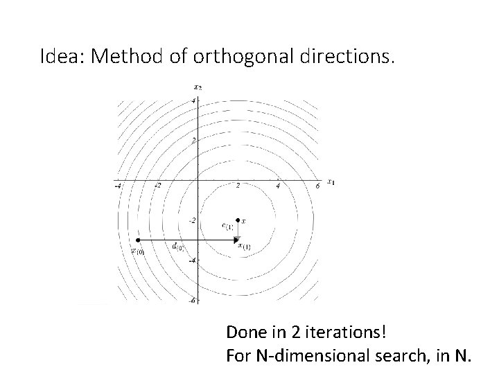
Idea: Method of orthogonal directions. Done in 2 iterations! For N-dimensional search, in N.

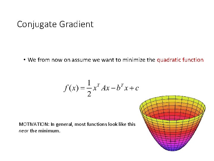
Conjugate Gradient • We from now on assume we want to minimize the quadratic function MOTIVATION: In general, most functions look like this near the minimum.

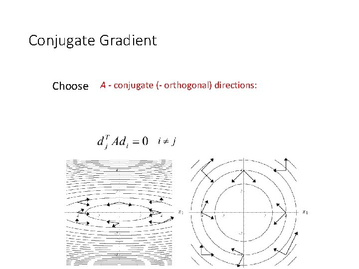
Conjugate Gradient Choose A - conjugate (- orthogonal) directions:

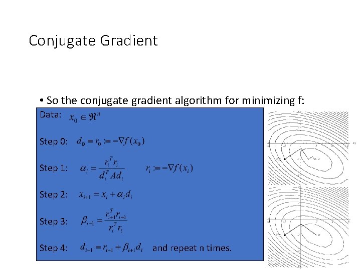
Conjugate Gradient • So the conjugate gradient algorithm for minimizing f: Data: Step 0: Step 1: Step 2: Step 3: Step 4: and repeat n times.

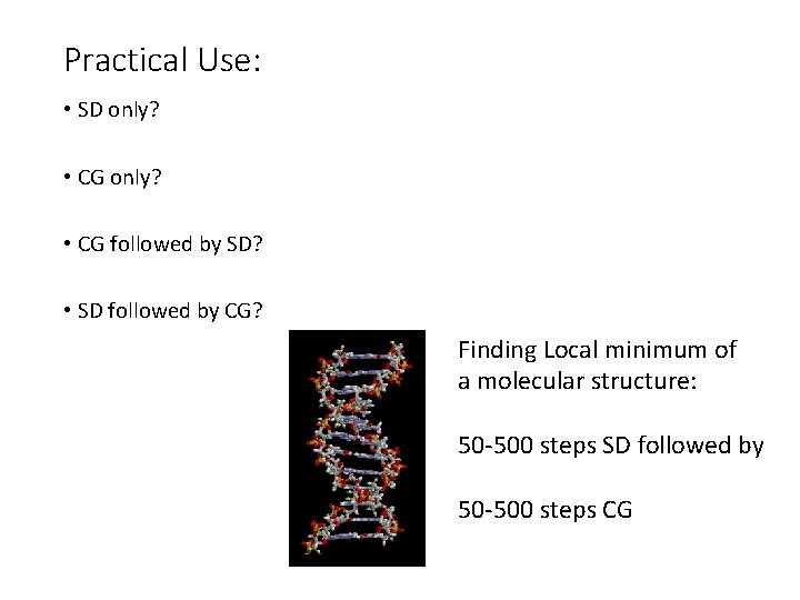
Practical Use: • SD only? • CG followed by SD? • SD followed by CG? Finding Local minimum of a molecular structure: 50 -500 steps SD followed by 50 -500 steps CG

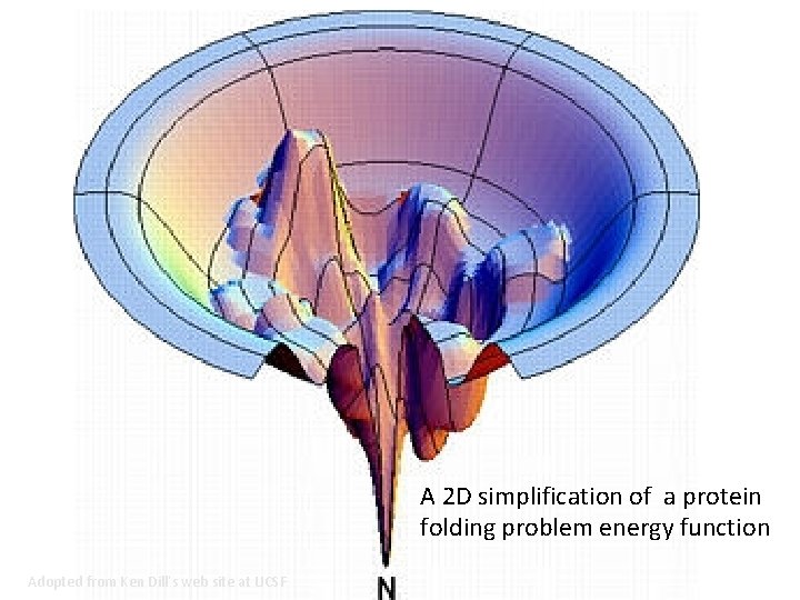
A 2 D simplification of a protein folding problem energy function Adopted from Ken Dill’s web site at UCSF

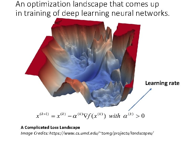
An optimization landscape that comes up in training of deep learning neural networks. Learning rate A Complicated Loss Landscape Image Credits: https: //www. cs. umd. edu/~tomg/projects/landscapes/

On to global optimization F[x_, y_] : = -Cos[5*x]*Cos[5*y]*Exp[-3*(x^2 + y^2)]; Global mimimum at (0, 0). A sure shot option: an exhaustive search. Define a fine enough grid (as above), start LOCAL (gradient) search from each grid point. Cost?

On to global optimization. • Cost of an exhaustive local search: • Say, 10 grid points in each dimension. Cost O(10 N). • Totally fine for N=1, 2, 3… • What about N=10? Or more?

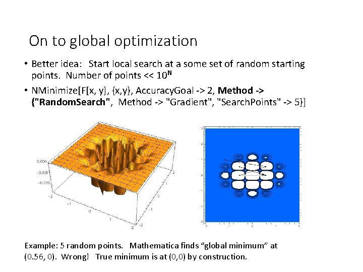
On to global optimization • Better idea: Start local search at a some set of random starting points. Number of points << 10 N • NMinimize[F[x, y], {x, y}, Accuracy. Goal -> 2, Method -> {"Random. Search", Method -> "Gradient", "Search. Points" -> 5}] Example: 5 random points. Mathematica finds “global minimum” at (0. 56, 0). Wrong! True minimum is at (0, 0) by construction.

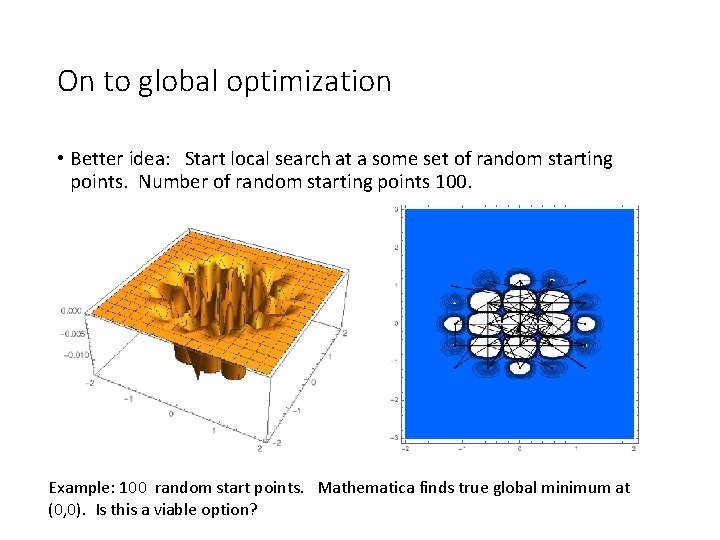
On to global optimization • Better idea: Start local search at a some set of random starting points. Number of random starting points 100. Example: 100 random start points. Mathematica finds true global minimum at (0, 0). Is this a viable option?

On to global optimization • For large N, even a million starting points will sample only a tiny subset of all 10 N relevant points. The global minimum will most likely be missed.