Supervised Learning Linear Models and Gradient Decent Algorithm

Supervised Learning Linear Models and Gradient Decent Algorithm

SUPERVISED LEARNING* • * https: //machinelearningmastery. com/supervised-and-unsupervised-machine-learning-algorithms/

SUPERVISED LEARNING • Supervised learning problems can be further grouped into regression and classification problems. • Classification: A classification problem is when the output variable is a category, such as “red” or “blue” or “disease” and “no disease”. • Regression: A regression problem is when the output variable is a real value, such as “dollars” or “weight”. • Some common types of problems built on top of classification and regression include recommendation and time series prediction respectively. • Some popular examples of supervised machine learning algorithms are: • Linear regression for regression problems. • Random forest for classification and regression problems. • Support vector machines for classification problems.

SUPERVISED LEARNING • A supervised learning algorithm analyzes the training data and produces an inferred function, which is called a classifier (if the output is discrete) or a regression function (if the output is continuous). • The inferred function should predict the correct output value for any valid input object. This requires the learning algorithm to generalize from the training data to unseen situations in a "reasonable" way.

SUPERVISED LEARNING • • Prediction Accuracy A good learner is the one which has good prediction accuracy; in other words, which has the smallest prediction error. Consider the simple case of fitting a linear regression model to the observed data. A model is a good fit, if it provides a high R 2 value. However, note that the model has used all the observed data and only the observed data. Hence, how it will perform when predicting for a new set of input values, is not clear. Assumption is that, with a high R 2 value, the model is expected to predict well for data observed in the future. Suppose now the model is more complex than a linear model and a spline smoother or a polynomial regression needs to be considered. What would be the proper complexity of the model? Would it be a fifth-degree polynomial or a cubic spline would suffice? Many modern classification and regression models are highly adaptable and are capable of formulating complex relationships. At the same time they may overemphasize patterns that are not reproducible. Without a methodological approach to evaluating models, the problem will not be detected until the next set of samples are predicted. And here we are not talking about the data quality of the sample, which is used to develop the model, being bad!

SUPERVISED LEARNING •

SUPERVISED LEARNING •

SUPERVISED LEARNING • A first issue is the tradeoff between bias and variance. • Imagine that we have available several different, but equally good, training data sets. • A learning algorithm is biased for a particular input x if, when trained on each of these data sets, it is systematically incorrect when predicting the correct output for x. • A learning algorithm has high variance for a particular input if it predicts different output values when trained on different training sets. • The prediction error of a learned classifier is related to the sum of the bias and the variance of the learning algorithm. • Generally, there is a tradeoff between bias and variance. A learning algorithm with low bias must be "flexible" so that it can fit the data well. But if the learning algorithm is too flexible, it will fit each training data set differently, and hence have high variance. • A key aspect of many supervised learning methods is that they are able to adjust this tradeoff between bias and variance (either automatically or by providing a bias/variance parameter that the user can adjust).

SUPERVISED LEARNING • The best learner is the one which can balance the bias and the variance of a model. For more information, you can visit https: //www. saylor. org/site/wp-content/uploads/2011/11/CS 405 -6. 2. 1. 2 -WIKIPEDIA. pdf

LINEAR MODELS AND GRADIENT DESCENT • Starting with an example • How do we predict housing prices • Collect data regarding housing prices and how they relate to size in feet Example problem: "Given this data, a friend has a house 750 square feet - how much can they be expected to get? "

• What approaches can we use to solve this? • Straight line through data • Maybe $150 000 • Second order polynomial • Maybe $200 000 • Each of these approaches represent a way of doing supervised learning • What does this mean? • We gave the algorithm a data set where a "right answer" was provided • So we know actual prices for houses • The idea is we can learn what makes the price a certain value from the training data • The algorithm should then produce more right answers based on new training data where we don't know the price already, i. e. predict the price • We also call this a regression problem • Predict continuous valued output (price) • No real discrete delineation

• What do we start with? Training set (this is your data set) • Notation m = number of training examples • x's = input variables / features • y's = output variable "target" variables • (x, y) - single training example • (xi, yj) - specific example (ith training example); i is an index to training set • With our training set defined - how do we used it? • Take training set • Pass into a learning algorithm • Algorithm outputs a function (denoted f ) (f = hypothesis) • This function takes an input (e. g. size of new house) • Tries to output the estimated value of Y

• How do we represent hypothesis f ? • Going to present f as; fθ(x) = θ 0 + θ 1 x • f(x) (shorthand) • What does this mean? • Means Y is a linear function of x! • θi are parameters • θ 0 is zero condition • θ 1 is gradient (slope) • This function is a linear regression with one variable • Also called simple linear regression • So in summary • A hypothesis takes in some variable • Uses parameters determined by a learning system • Outputs a prediction based on that input

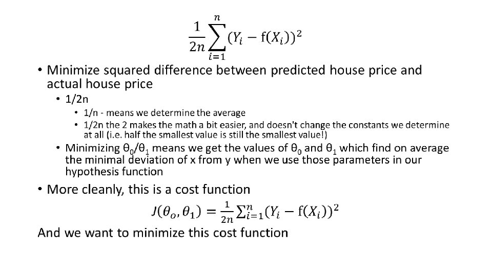
Linear regression - implementation (cost function) • A cost function lets us figure out how to fit the best straight line to our data. • Choosing values for θi (parameters) • Different values give you different functions • If θ 0 is 1. 5 and θ 1 is 0 then we get straight line parallel with X along 1. 5 @ y • If θ 1 is > 0 then we get a positive slope • Based on our training set we want to generate parameters which make the straight line • Chosen these parameters so fθ(x) is close to y for our training examples • Basically, uses x’s in training set with fθ(x) to give output which is as close to the actual y value as possible • Think of fθ(x) as a "y imitator" - it tries to convert the x into y, and considering we already have y we can evaluate how well fθ(x) does this • To formalize this; • We want to solve a minimization problem • Minimize (fθ(x) - y)2 • i. e. minimize the difference between f(x) and y for each/any/every example • Sum this over the training set

• Cost Function

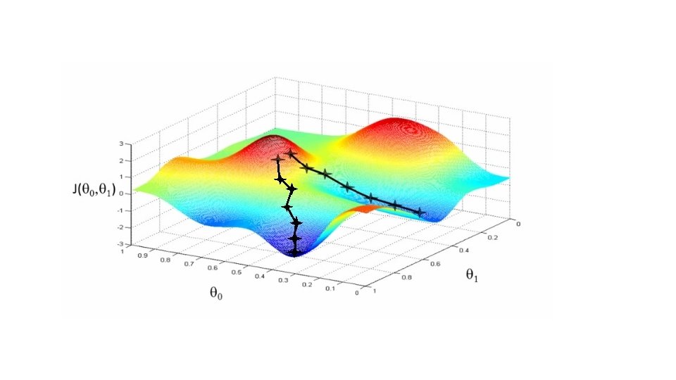
• We can see that the height (y) indicates the value of the cost function, so find where y is at a minimum • Instead of a surface plot we can use a contour figures/plots • Set of ellipses in different colors • Each color is the same value of J(θ 0, θ 1), but obviously plot to different locations because θ 1 and θ 0 will vary • Imagine a bowl shape function coming out of the screen so the middle is the concentric circles

• Each point (like the red one above) represents a pair of parameter values for Ɵ 0 and Ɵ 1 • Our example here put the values at • θ 0 = ~800 • θ 1 = ~-0. 15 • Not a good fit • i. e. these parameters give a value on our contour plot far from the center • If we have • θ 0 = ~360 • θ 1 = 0 • This gives a better hypothesis, but still not great - not in the center of the contour plot • Finally we find the minimum, which gives the best hypothesis • Doing this by eye/hand is hard • What we really want is an efficient algorithm for finding the minimum for θ 0 and θ 1

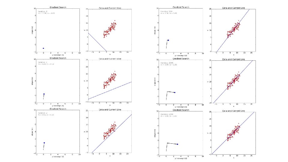
GRADIENT DESCENT ALGORITHM • At a theoretical level, gradient descent is an algorithm that minimizes functions. Given a function defined by a set of parameters, gradient descent starts with an initial set of parameter values and iteratively moves toward a set of parameter values that minimize the function. This iterative minimization is achieved using calculus, taking steps in the negative direction of the function gradient. • Minimize cost function J • Gradient descent • Used all over machine learning for minimization • Start by looking at a general J() function • Problem • We have J(θ 0, θ 1) • We want to get min J(θ 0, θ 1) • Gradient descent applies to more general functions • J(θ 0, θ 1, θ 2. . θp) • min J(θ 0, θ 1, θ 2. . θp)

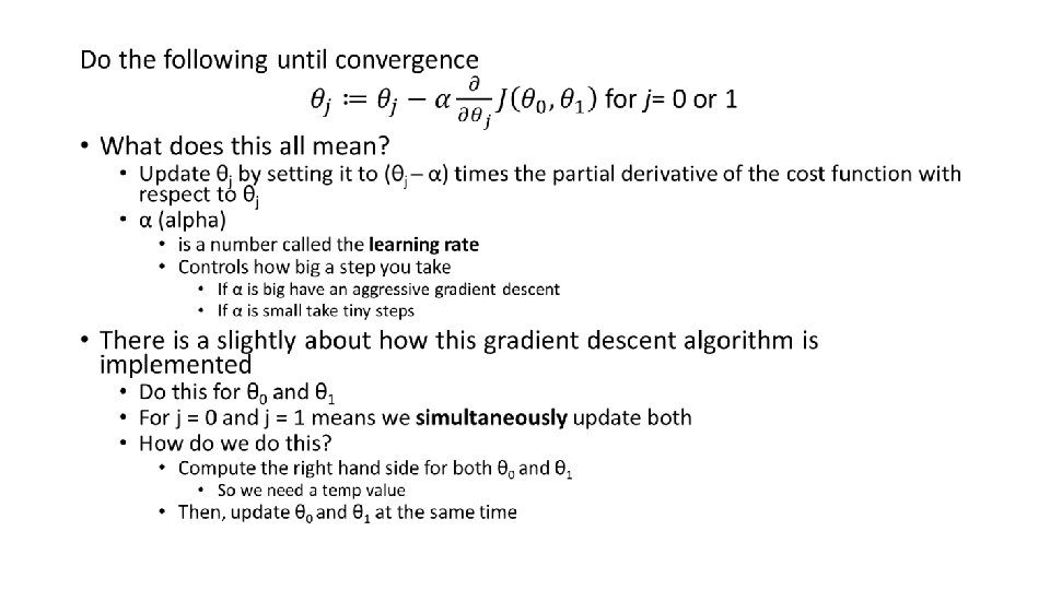
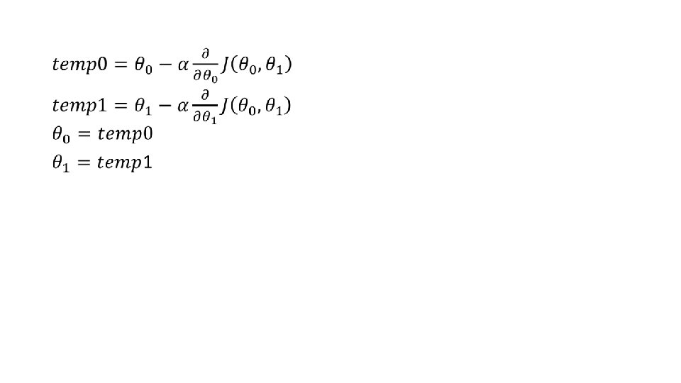
How does it work? • Start with initial guesses • Start at 0, 0 (or any other value) • Keeping changing θ 0 and θ 1 a little bit to try and reduce J(θ 0, θ 1) • Each time you change the parameters, you select the gradient which reduces J(θ 0, θ 1) the most possible • Repeat • Do so until you converge to a local minimum • Has an interesting property • Where you start can determine which minimum you end up

STEPS IN THE GRADIENT DESCENT ALGORITHM* • Lets now go step by step to understand the Gradient Descent algorithm: • Step 1: Initialize the weights ( 0 and 1) with random values and calculate Error (SSE) • Step 2: Calculate the gradient i. e. change in SSE when the weights ( 0 and 1) are changed by a very small value from their original randomly initialized value. This helps us move the values of 0 and 1 in the direction in which SSE is minimized. • Step 3: Adjust the weights with the gradients to reach the optimal values where SSE is minimized • Step 4: Use the new weights for prediction and to calculate the new SSE • Step 5: Repeat steps 2 and 3 till further adjustments to weights doesn’t significantly reduce the Error * https: //www. kdnuggets. com/2017/04/simple-understand-gradient-descent-algorithm. html

Gradient descent over multi-dimensional parameters •

EXAMPLE • We will now go through each of the steps in detail. But before that, we have to standardize the data as it makes the optimization process faster.

Step 1: To fit a line Ypred = a + b X, start off with random values of a and b and calculate prediction error (SSE)

Step 2: Calculate the error gradient w. r. t the weights ∂SSE/∂a = – (Y-YP) ∂SSE/∂b = – (Y-YP)X Here, SSE=½ (Y-YP)2 = ½(Y-(a+b. X))2 ∂SSE/∂a and ∂SSE/∂b are the gradients and they give the direction of the movement of a, b w. r. t to SSE.

Step 3: Adjust the weights with the gradients to reach the optimal values where SSE is minimized We need to update the random values of a, b so that we move in the direction of optimal a, b. Update rules: a – ∂SSE/∂a b – ∂SSE/∂b So, update rules: New a = a – α * ∂SSE/∂a = 0. 45 -0. 01*3. 300 = 0. 42 New b = b – α * ∂SSE/∂b= 0. 75 -0. 01*1. 545 = 0. 73 Here, α is the learning rate = 0. 01, which is the pace of adjustment to the weights.

Step 4: Use new a and b for prediction and to calculate new Total SSE You can see with the new prediction, the total SSE has gone down (0. 677 to 0. 553). That means prediction accuracy has improved. Step 5: Repeat step 3 and 4 till the time further adjustments to a and b doesn’t significantly reduces the error. At that time, we have arrived at the optimal a and b with the highest prediction accuracy. • This is the Gradient Descent Algorithm. This optimization algorithm and its variants form the core of many machine learning algorithms like Neural Networks and even Deep Learning.

While we were able to scratch the surface for learning gradient descent, there are several additional concepts that are good to be aware of that we weren’t able to discuss. A few of these include: • Convexity – In our linear regression problem, there was only one minimum. Our error surface was convex. Regardless of where we started, we would eventually arrive at the absolute minimum. In general, this need not be the case. It’s possible to have a problem with local minima that a gradient search can get stuck in. There are several approaches to mitigate this (e. g. , stochastic gradient search). • Performance – We used vanilla gradient descent with a learning rate of 0. 0005, and ran it for 2000 iterations. There approaches such a line search, that can reduce the number of iterations required. For the above example, line search reduces the number of iterations to arrive at a reasonable solution from several thousand to around 50. • Convergence – How to determine when the search finds a solution is typically done by looking for small changes in error iteration-to-iteration (e. g. , where the gradient is near zero).

• We have an almost identical rule for multivariate gradient descent • Polynomial regression for non-linear function • Example • House price prediction • Two features • Frontage - width of the plot of land along road (x 1) • Depth - depth away from road (x 2) • You don't have to use just two features • Can create new features • Might decide that an important feature is the land area • So, create a new feature = frontage * depth (x 3) • h(x) = θ 0 + θ 1 x 3 • Area is a better indicator • Often, by defining new features you may get a better model • Polynomial regression • May fit the data better • θ 0 + θ 1 x + θ 2 x 2 e. g. here we have a quadratic function • For housing data could use a quadratic function • But may not fit the data so well - inflection point means housing prices decrease when size gets really big • So instead must use a cubic function

• How do we fit the model to this data • To map our old linear hypothesis and cost functions to these polynomial descriptions the easy thing to do is set • x 1 = x • x 2 = x 2 • x 3 = x 3 • By selecting the features like this and applying the linear regression algorithms you can do polynomial linear regression • Remember, feature scaling becomes even more important here • Instead of a conventional polynomial you could do variable ^(1/something) - i. e. square root, cubed root etc.

R APPLICATION OF THE GRADIENT DECENT ALGORITHM attach(mtcars) plot(disp, mtcars[, 1], col = "blue", pch = 20) > model <- lm(mtcars[, 1] ~ disp, data = mtcars) > coef(model) (Intercept) disp 29. 59985476 -0. 04121512

y_preds <- predict(model) abline(model) > errors <- unname((mtcars[, 1] - y_preds) ^ 2) > sum(errors) / length(mtcars[, 1]) [1] 9. 911209

gradient. Desc <- function(x, y, learn_rate, conv_threshold, n, max_iter) { plot(x, y, col = "blue", pch = 20) m <- runif(1, 0, 1) c <- runif(1, 0, 1) yhat <- m * x + c MSE <- sum((y - yhat) ^ 2) / n converged = F iterations = 0 while(converged == F) { ## Implement the gradient descent algorithm m_new <- m - learn_rate * ((1 / n) * (sum((yhat - y) * x))) c_new <- c - learn_rate * ((1 / n) * (sum(yhat - y))) m <- m_new c <- c_new yhat <- m * x + c MSE_new <- sum((y - yhat) ^ 2) / n if(MSE - MSE_new <= conv_threshold) { abline(c, m) converged = T return(paste("Optimal intercept: ", c, "Optimal slope: ", m)) } iterations = iterations + 1 if(iterations > max_iter) { abline(c, m) converged = T return(paste("Optimal intercept: ", c, "Optimal slope: ", m, “MSE”, MSE_new)) } } }

# Run the function > gradient. Desc(disp, mtcars[, 1], 0. 0000293, 0. 001, 32, 2500000) [1] "Optimal intercept: 29. 5998515131943 Optimal slope: 0. 0412151089777685 MSE 9. 91120904007057“ > coef(model) (Intercept) disp 29. 59985476 -0. 04121512

STOCHASTIC GRADIENT DESCENT •

STOCHASTIC GRADIENT DESCENT •

LINEAR REGRESSION APPLICATION (https: //towardsdatascience. com/step-by-step-tutorial-on-linear-regression-with-stochastic-gradient-descent-1 d 35 b 088 a 843 ) • We have some data: as we observe the independent variables x₁ and x₂, we observe the dependent variable (or response variable) y along with it. • In our dataset, we have 6 examples (or observations). x 1 x 2 y 1) 4 1 2 2) 2 8 -14 3) 1 0 1 4) 3 2 -1 5) 1 4 -7 6) 6 7 -8

Model • The next question to ask: “How are both x₁ and x₂ related to y? ” • We believe that they are connected to each other by this equation: • our job today is to find the ‘best’ w and b values. • The deep learning conventions w and b, which stand for weights and biases respectively. But note that linear regression is not deep learning.

Define loss function • Let’s say at the end of this exercised, we’ve figured out our model to be • How do we know if our model is doing well? • We simply compare the predicted ŷ and the observed y through a loss function. There are many ways to define the loss function but in this post, we define it as the squared difference between ŷ and y. • Generally, the smaller the L, the better.

Minimize loss function • Because we want the difference between ŷ and y to be small, we want to make an effort to minimize it. This is done through stochastic gradient descent optimization. It is basically iteratively updating the values of w₁ and w₂ using the value of gradient, as in this equation: • This algorithm tries to find the right weights by constantly updating them, bearing in mind that we are seeking values that minimize the loss function.

Implementation • The workflow for training our model is simple: forward propagation (or feed-forward or forward pass) and backpropagation. • Training just means regularly updating the values of your weights, put simply.

STEP 0. Build computation graph • To keep track of all the values, we build a ‘computation graph’ that comprises nodes color-coded in • • orange — the placeholders (x₁, x₂ and y), dark green — the weights and bias (w₁, w₂ and b), light green — the model (ŷ) connecting w₁, w₂, b, x₁ and x₂, and yellow — the loss function (L) connecting the ŷ and y. For forward propagation, you should read this graph from top to bottom and for backpropagation bottom to top. Fig. 0: Computation graph for linear regression model with stochastic gradient descent.

STEP 1. Forward Propagation: Initialize weights (one-time) • Since gradient descent is all about updating the weights, we need them to start with some values, known as initializing weights. • Here we initialized the weights and bias as follows: In this example, we initialized the weights by using truncated normal distribution and the bias with 0. Fig. 1: Weights initialized (dark green nodes)

STEP 2. Forward Propagation: Feed data • We set the batch size to be 1 and we feed in this first batch of data. • Batch and batch size: We can divide our dataset into smaller groups of equal size. Each group is called a batch and consists of a specified number of examples, called batch size. If we multiply these two numbers, we should get back the number of observations in our data. • Here, our dataset consists of 6 examples and since we defined the batch size to be 1 in this training, we have 6 batches altogether. Eqn. 1: First batch of data fed into model Fig. 2. 2: Feeding data to model with first batch (orange nodes)

STEP 3. Forward Propagation: Compute ŷ • Now that we have the values of x₁, x₂, w₁, w₂ and b ready, let’s compute ŷ. • The value of ŷ (= 0. 1) is reflected in the light green node below: Fig. 3: ŷ computed (light green node)

Fig. 4. 1: L computed (yellow node) Eqn. 2: Compute the loss Fig. 4. 1: L computed (yellow node) It is a common practice to log the loss during training, together with other information like the epoch, batch and time taken.

STEP 5: Backpropagation: Compute partial differentials • Before we start adjusting the values of the weights and bias w₁, w₂ and b, let’s first compute all the partial differentials. These are needed later when we do the weight update. • Namely, we compute all possible paths leading to every w and b only, because these are the only variables which we are interested in updating. • From Fig. 5, we see that there are 4 edges that we labeled with the partial differentials. Fig. 5: Indicated partial differentials to the relevant edges on the graph

• Recall the equations for the model and loss function: Model Loss • The partial differentials are as follows: L (yellow) — ŷ (light green): ŷ (light green) — b (dark green): ŷ (light green) — w₁ (dark green): ŷ (light green) — w₂ (dark green):

STEP 6. Backpropagation: Update weights • Observe the dark green nodes in Fig. 6 below. We see three things: i) b changes from 0. 000 to 0. 212 ii) w₁ changes from 0. 017 to 0. 829 iii) w₂ changes from 0. 048 to 0. 164 Fig. 6: Updating the weights and bias (dark green nodes)

• This is stochastic gradient descent — updating the weights using backpropagation, making use of the respective gradient values. • Let’s first focus on updating b. The formula for updating b is Stochastic gradient descent update for b where b — current value b’ — value after update η —learning rate, set to 0. 05 ∂L/∂b — gradient i. e. partial differential of L w. r. t. b

• To get the gradient, we need to multiply the paths from L leading to b using chain rule: • We would require the current batch values of x, y, ŷ and the partial differentials so let’s just place them below for easy reference: Values from current batch and the predicted ŷ

• Using the stochastic gradient descent equation and plucking in all the values gives us That’s it for updating b! We are left with updating w₁ and w₂, which we update in a similar fashion. End of batch iteration Congrats! That’s it for dealing with the first batch!

• Now we need to iterate the above-mentioned steps to the other 5 batches, namely examples 2 to 6.

End of epoch • We complete 1 epoch when the model has iterated through all the batches once. In practice, we extend the epoch to more than 1. • One epoch is when our setup has seen all the observations in our dataset once. But one epoch is almost always never enough for the loss to converge. In practice, this number is manually tuned. • At the end of it all, you should get a final model, ready for inference, say:

Improve training • One epoch is never enough for a stochastic gradient descent optimization problems. Remember that our first loss value is at 4. 48. If we increase the number of epochs, which means just increasing the number of times we update the weights and biases, we can converge it to a satisfactory low. • Below are things you can improve the training: • • • Extend training to more than 1 epoch Increase batch size Change optimizer Adjust learning rate (changing the learning rate value or using learning rate schedulers) Hold out a train-validation-test set

Logistic Regression As a Classification Tool • Where Y is a discrete value • Develop the logistic regression algorithm to determine what class a new input should fall into • Classification problems • Email -> spam/not spam? • Online transactions -> fraudulent? • Tumor -> Malignant/benign • Variable in these problems is Y • Y is either 0 or 1 • 0 = negative class (absence of something) • 1 = positive class (presence of something) • Start with binary class problems • How do we develop a classification algorithm? • Tumor size vs malignancy (0 or 1) • We could use linear regression • Then threshold the classifier output (i. e. anything over some value is yes, else no) • In our example below linear regression with thresholding seems to work

• We can see above this does a reasonable job of stratifying the data points into one of two classes • But what if we had a single Yes with a very small tumour • This would lead to classifying all the existing yeses as nos • Another issues with linear regression • We know Y is 0 or 1 • Hypothesis can give values large than 1 or less than 0 • So, logistic regression generates a value where is always either 0 or 1 • Logistic regression is a classification algorithm - don't be confused

HYPOTHESIS REPRESENTATION •

• What does the sigmoid function look like • Crosses 0. 5 at the origin, then flattens out] • Asymptotes at 0 and 1 • Given this we need to fit θ to our data Interpreting hypothesis output • When our hypothesis (hθ(x)) outputs a number, we treat that value as the estimated probability that y=1 on input x • Example • If X is a feature vector with x 0 = 1 (as always) and x 1 = tumor. Size • hθ(x) = 0. 7 Tells a patient they have a 70% chance of a tumor being malignant • We can write this using the following notation hθ(x) = P(y=1|x ; θ) • What does this mean? Probability that y=1, given x, parameterized by θ • Since this is a binary classification task we know y = 0 or 1 • So the following must be true • P(y=1|x ; θ) + P(y=0|x ; θ) = 1 • P(y=0|x ; θ) = 1 - P(y=1|x ; θ)

DECISION BOUNDARY • Gives a better sense of what the hypothesis function is computing • Better understand of what the hypothesis function looks like • One way of using the sigmoid function is; • When the probability of y being 1 is greater than 0. 5 then we can predict y = 1 • Else we predict y = 0 • When is it exactly that hθ(x) is greater than 0. 5? • Look at sigmoid function • g(z) is greater than or equal to 0. 5 when z is greater than or equal to 0

hθ(x) = g(θ 0 + θ 1 x 1 + θ 2 x 2) • So, for example • θ 0 = -3 • θ 1 = 1 • θ 2 = 1 • So our parameter vector is a column vector with the above values • So, θT is a row vector = [-3, 1, 1] • What does this mean? • The z here becomes θT x • We predict "y = 1" if • -3 x 0 + 1 x 1 + 1 x 2 >= 0 • -3 + x 1 + x 2 >= 0

• We can also re-write this as • If (x 1 + x 2 >= 3) then we predict y = 1 • If we plot • x 1 + x 2 = 3 we graphically plot our decision boundary Means we have these two regions on the graph Blue = false Magenta = true Line = decision boundary Concretely, the straight line is the set of points where hθ(x) = 0. 5 exactly The decision boundary is a property of the hypothesis Means we can create the boundary with the hypothesis and parameters without any data Later, we use the data to determine the parameter values i. e. y = 1 if 5 - x 1 > 0 5 > x 1

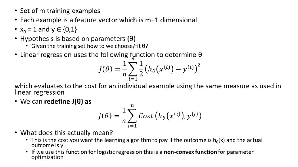
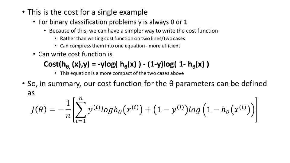
Cost function for logistic regression •

• What do we mean by non convex? • We have some function - J(θ) - for determining the parameters • Our hypothesis function has a non-linearity (sigmoid function of hθ(x) ) • This is a complicated non-linear function • If you take hθ(x) and plug it into the Cost() function, and them plug the Cost() function into J(θ) and plot J(θ) we find many local optimum -> non convex function • Why is this a problem • Lots of local minima mean gradient descent may not find the global optimum - may get stuck in a global minimum • We would like a convex function so if you run gradient descent you converge to a global minimum

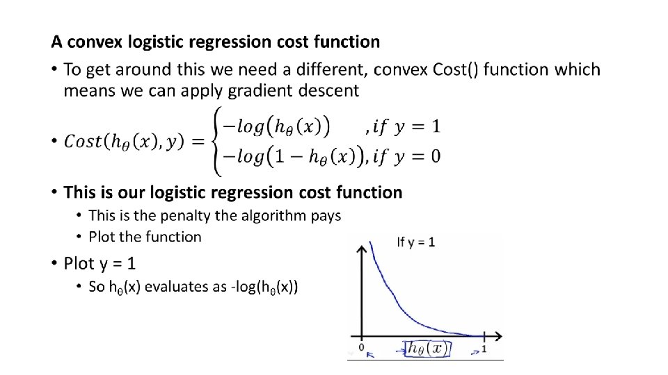
• So when we're right, cost function is 0 • Else it slowly increases cost function as we become "more" wrong • X axis is what we predict • Y axis is the cost associated with that prediction • This cost functions has some interesting properties • If y = 1 and hθ(x) = 1 • If hypothesis predicts exactly 1 and that’s exactly correct then that corresponds to 0 (exactly, not nearly 0) • As hθ(x) goes to 0 • Cost goes to infinity • This captures the intuition that if hθ(x) = 0 (predict P (y=1|x; θ) = 0) but y = 1 this will penalize the learning algorithm with a massive cost

• What about if y = 0 • then cost is evaluated as -log(1 - hθ( x )) • Just get inverse of the other function • Now it goes to plus infinity as hθ(x) goes to 1 • With our particular cost functions J(θ) is going to be convex and avoid local minimum

Simplified cost function and gradient descent •

• Why do we chose this function when other cost functions exist? • This cost function can be derived from statistics using the principle of maximum likelihood estimation • Also has the nice property that it's convex • To fit parameters θ: • Find parameters θ which minimize J(θ) • This means we have a set of parameters to use in our model for future predictions

How to minimize the logistic regression cost function •

R APPLICATION Suppose that you are an administrator of a university and you want to know the chance of admission of each applicant based on their two exams. You have historical data from previous applicants which can be used as the training data for logistic regression. Your task is to build a classification model that estimates each applicant’s probability of admission in university (Source: coursera machine learning class and https: //www. r-bloggers. com/logistic-regression-with-r-step-by-stepimplementation-part-2/ ).

> #Load data (https: //www. r-bloggers. com/logistic-regression-with-r -step-by-step-implementation-part-2/) > data <- read. csv("data. csv") > #Create plot >plot(data$score. 1, data$score. 2, col=as. factor(data$label), xlab="Sco re-1", ylab="Score-2")

So, in this case we have two predictor variables (two exams’ scores) and label as response variable. Let us set predictor and response variables. #Predictor variables X <- as. matrix(data[, c(1, 2)]) #Add ones to X X <- cbind(rep(1, nrow(X)), X) #Response variable Y <- as. matrix(data$label) Our first step is to implement sigmoid function. #Sigmoid function sigmoid <- function(z) { g <- 1/(1+exp(-z)) return(g) }

Let’s test this cost function with initial theta parameters. We will set theta parameters equal to zero initially and check the cost. > #Intial theta > initial_theta <- rep(0, ncol(X)) > > #Cost at inital theta > cost(initial_theta) [1] 0. 6931472 You will find cost is 0. 693 with initial parameters. Now, our objective is to minimize this cost and derive the optimal value of thetas. Amar Gondaliya (blog owner) implemented gradient descent and defined the update function to optimize the values of theta. He used optim() to derive the best fitting parameters. Ultimately we want to have optimal value of the cost function and theta.

> # Derive theta using gradient descent using optim function > theta_optim <- optim(par=initial_theta, fn=cost) > #set theta > theta <- theta_optim$par > #cost at optimal value of theta > theta_optim$value [1] 0. 2034977 • We have optimal values of theta and cost is about 0. 2034 at optimal value of theta. We can now use this theta parameter for predicting for the admission probability for new applicant based on the score of two exams. • For example, a student is with exam-1 score of 45 and exam-2 score of 85. > # probability of admission for student > prob <- sigmoid(t(c(1, 45, 85))%*%theta) > prob [, 1] [1, ] 0. 7763541

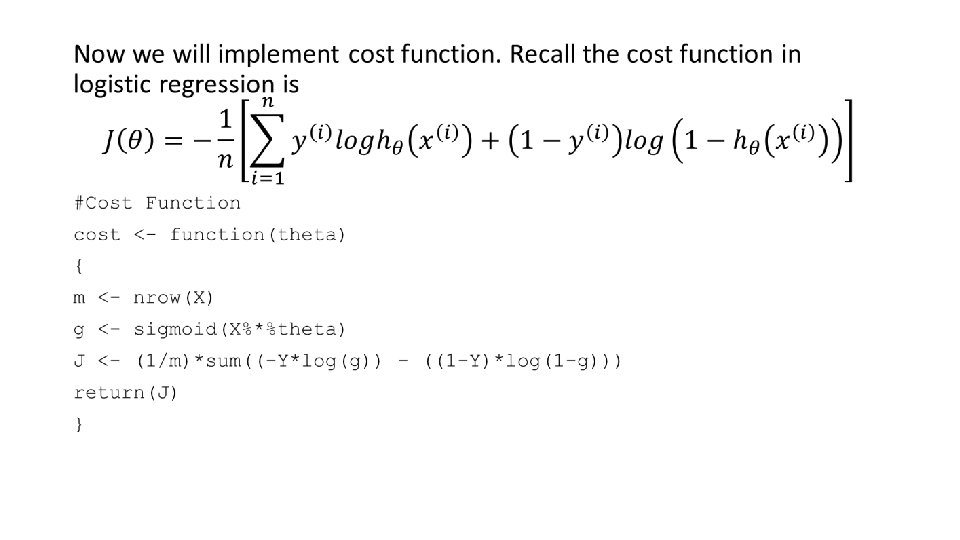
#ex 2 logistic regression Data 1 <- read. csv("data. csv") colnames(Data 1) = c("exam 1", "exam 2", "admit") #plot the data with(Data 1, plot(exam 1[admit==1], exam 2[admit==1])) with(Data 1, points(exam 1[admit==0], exam 2[admit==0], col="red")) # sigmoid function sigmoid = function(z){ 1 / (1 + exp(-z)) } #cost function cost = function(X, y, theta){ m = nrow(X) hx = sigmoid(X %*% theta) (1/m) * (((-t(y) %*% log(hx)) - t(1 -y) %*% log(1 - hx))) }

#gradient grad = function(X, y, theta){ m = nrow(X) hx = sigmoid(X %*% theta) (1/m) * (t(X) %*% (hx - y)) } #gradient descent alpha = 0. 001 maxinteration = 6000000 #lm(y ~ X) theta = matrix(c(-1. 3, 0. 01), nrow=3) m = nrow(Data 1) y = as. matrix(Data 1[, 3]) X = as. matrix(Data 1[, c(1, 2)]) X = cbind(1, X) for (i in 1: maxinteration){ theta = theta - alpha * grad(X, y, theta) } print(theta) [, 1] -23. 7000448 exam 1 0. 1945461 exam 2 0. 1896456 For a student is with exam-1 score of 45 and exam-2 score of 85, probability that he/she will be accepted is 0. 7629. m 1=glm(Data 1[, 3]~ Data 1[, 1]+ Data 1[, 2], family="binomial") summary(m 1) Coefficients: (Intercept) Data 1[, 1] Data 1[, 2] -25. 1613 0. 2062 0. 2015 For a student is with exam-1 score of 45 and exam-2 score of 85, probability that he/she will be accepted is 0. 7765.

• To see different types of gradient descent algorithms, you can visit http: //ruder. io/optimizing-gradientdescent/index. html#stochasticgradientdescent