Lecture 4 Model Selection and Multimodel Inference Topics

Lecture 4 Model Selection and Multimodel Inference

Topics l Model selection: how do you choose between (and compare) alternate models? l Multimodel inference: how do you combine information from more than 1 model?

Comparing alternative models l We don’t ask “Is the model right or wrong? ” We ask “Do the data support one model more than a competing model? ” l Strength of evidence (support) for a model is relative: - Relative to other models: As models improve, - support may change. Relative to data at hand: As the data improve, support may change.

But is likelihood enough? The challenge of parsimony The importance of seeking simple answers. . . “It will not be sufficient, when faced with a mass of observations, to plead special creation, even though, as we shall see, such a hypothesis commands a higher numerical likelihood than any other. ” (Edwards, 1992, pg. 1, in explaining the need for a rigorous basis for scientific inference, given uncertainty in nature. . . )

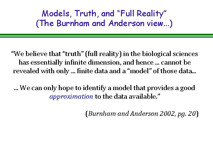
Models, Truth, and “Full Reality” (The Burnham and Anderson view. . . ) “We believe that “truth” (full reality) in the biological sciences has essentially infinite dimension, and hence. . . cannot be revealed with only. . . finite data and a “model” of those data. . . We can only hope to identify a model that provides a good approximation to the data available. ” (Burnham and Anderson 2002, pg. 20)

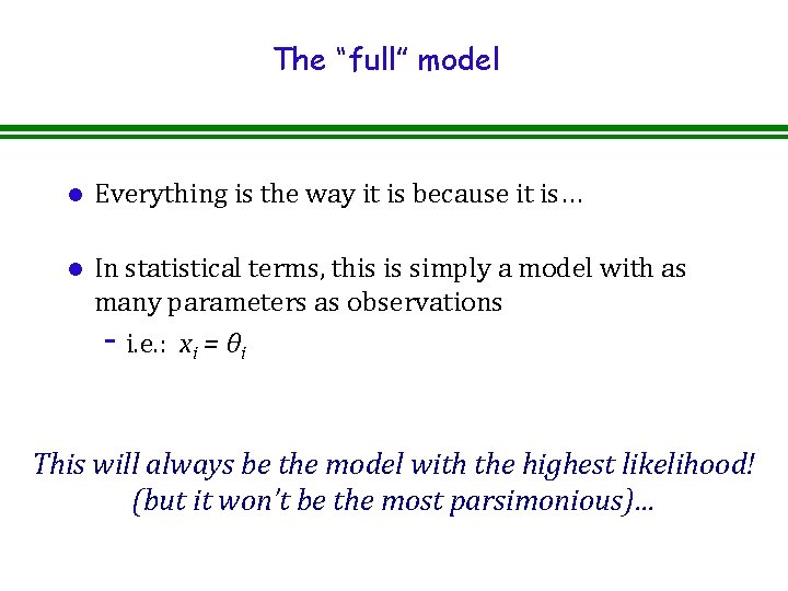
The “full” model l Everything is the way it is because it is… l In statistical terms, this is simply a model with as many parameters as observations - i. e. : xi = θi This will always be the model with the highest likelihood! (but it won’t be the most parsimonious)…

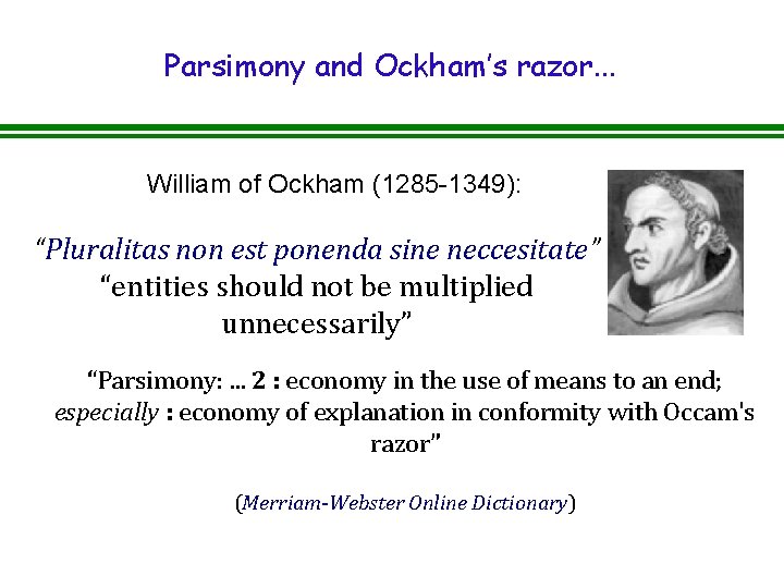
Parsimony and Ockham’s razor. . . William of Ockham (1285 -1349): “Pluralitas non est ponenda sine neccesitate” “entities should not be multiplied unnecessarily” “Parsimony: . . . 2 : economy in the use of means to an end; especially : economy of explanation in conformity with Occam's razor” (Merriam-Webster Online Dictionary)

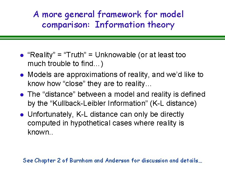
A more general framework for model comparison: Information theory l l “Reality” = “Truth” = Unknowable (or at least too much trouble to find…) Models are approximations of reality, and we’d like to know how “close” they are to reality… The “distance” between a model and reality is defined by the “Kullback-Leibler Information” (K-L distance) Unfortunately, K-L distance can only be directly computed in hypothetical cases where reality is known. . See Chapter 2 of Burnham and Anderson for discussion and details…

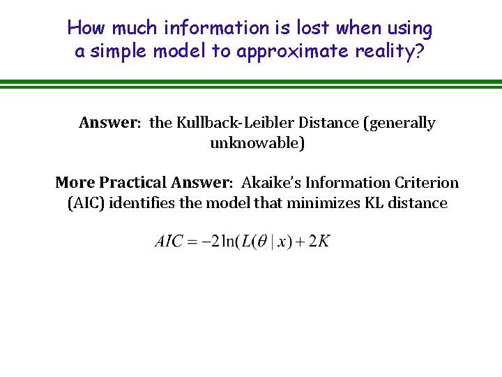
How much information is lost when using a simple model to approximate reality? Answer: the Kullback-Leibler Distance (generally unknowable) More Practical Answer: Akaike’s Information Criterion (AIC) identifies the model that minimizes KL distance

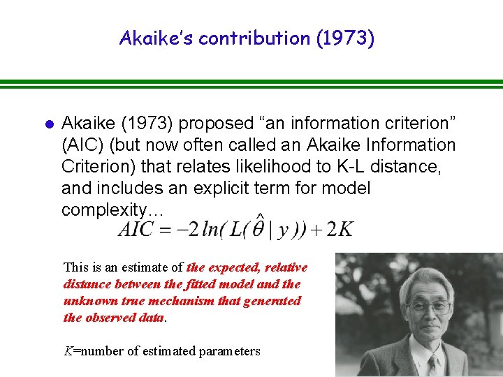
Akaike’s contribution (1973) l Akaike (1973) proposed “an information criterion” (AIC) (but now often called an Akaike Information Criterion) that relates likelihood to K-L distance, and includes an explicit term for model complexity… ^ This is an estimate of the expected, relative distance between the fitted model and the unknown true mechanism that generated the observed data. K=number of estimated parameters

General guidelines for use of AIC l We select the model with smallest value of AIC (i. e. closest to “truth”). l AIC will identify the best model in the set, even if all the models are poor! l It is the researcher’s (your) responsibility that the set of candidate models includes well founded, realistic models.

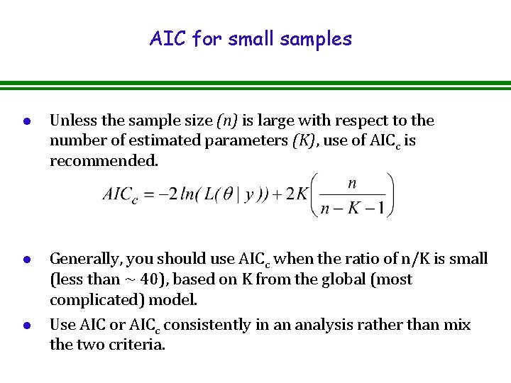
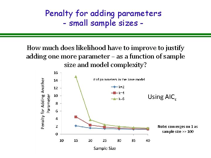
AIC for small samples l Unless the sample size (n) is large with respect to the number of estimated parameters (K), use of AICc is recommended. l Generally, you should use AICc when the ratio of n/K is small (less than ~ 40), based on K from the global (most complicated) model. Use AIC or AICc consistently in an analysis rather than mix the two criteria. l

Penalty for adding parameters - small sample sizes How much does likelihood have to improve to justify adding one more parameter – as a function of sample size and model complexity? Using AICc Note: converges on 1 as sample size >> 100

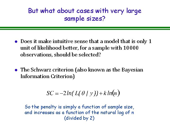
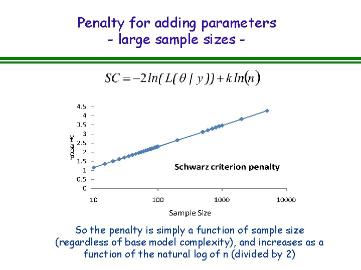
But what about cases with very large sample sizes? l Does it make intuitive sense that a model that is only 1 unit of likelihood better, for a sample with 10000 observations, should be selected? l The Schwarz criterion (also known as the Bayesian Information Criterion) So the penalty is simply a function of sample size, and increases as a function of the natural log of n (divided by 2)

Penalty for adding parameters - large sample sizes - So the penalty is simply a function of sample size (regardless of base model complexity), and increases as a function of the natural log of n (divided by 2)

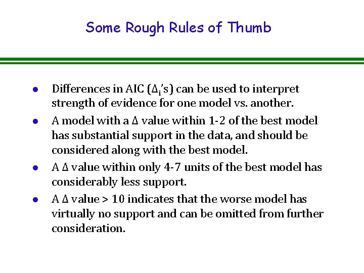
Some Rough Rules of Thumb l l Differences in AIC (Δi’s) can be used to interpret strength of evidence for one model vs. another. A model with a Δ value within 1 -2 of the best model has substantial support in the data, and should be considered along with the best model. A Δ value within only 4 -7 units of the best model has considerably less support. A Δ value > 10 indicates that the worse model has virtually no support and can be omitted from further consideration.

Comparing models with different PDFs l LRTs and AIC can be used as one basis for selecting the “best” PDF for a given dataset and model, l But more generally, an examination of the distribution of the residuals should guide the choice of the appropriate PDF l There will be cases where different PDFs are appropriate for different models applied to the same dataset - Example: neighborhood competition models where residuals shift from lognormally to normally distributed as the models are improved by additional terms

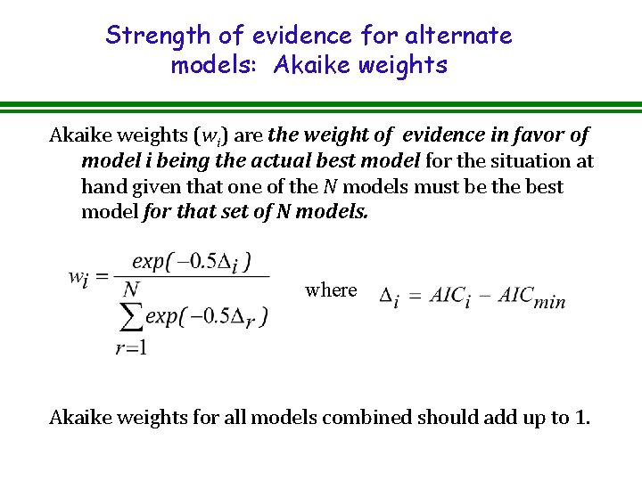
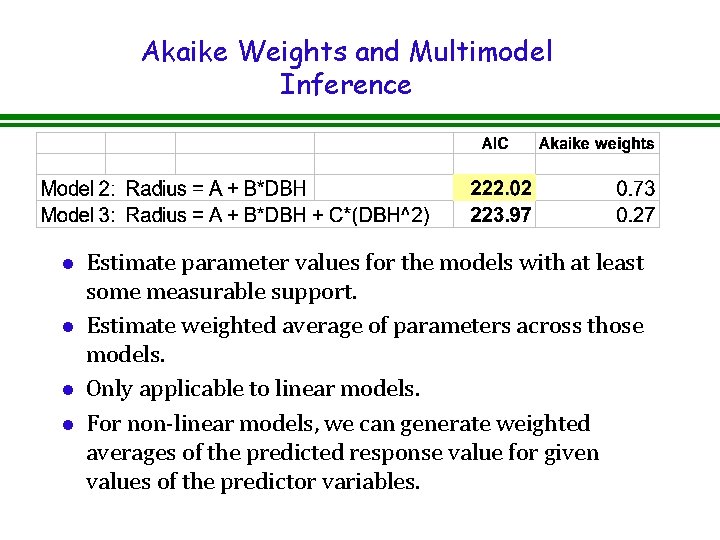
Strength of evidence for alternate models: Akaike weights (wi) are the weight of evidence in favor of model i being the actual best model for the situation at hand given that one of the N models must be the best model for that set of N models. where Akaike weights for all models combined should add up to 1.

Uses of Akaike weights l “Probability” that the candidate model is the best model. l Relative strength of evidence (evidence ratios). l Variable selection—which independent variable has the greatest influence? l Model averaging.

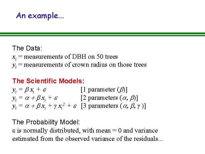
An example. . . The Data: xi = measurements of DBH on 50 trees yi = measurements of crown radius on those trees The Scientific Models: yi = b xi + e [1 parameter (b)] yi = a + b xi + e [2 parameters (a, b)] yi = a + b xi + γ xi 2 + e [3 parameters (a, b, γ )] The Probability Model: e is normally distributed, with mean = 0 and variance estimated from the observed variance of the residuals. . .

Back to the example…. . Akaike weights can be interpreted as the estimated probability that model i is the best model for the data at hand, given the set of models considered. Weights > 0. 90 indicate that robust inferences can be made using just that model.

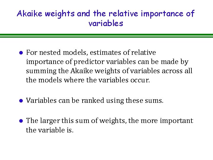
Akaike weights and the relative importance of variables l For nested models, estimates of relative importance of predictor variables can be made by summing the Akaike weights of variables across all the models where the variables occur. l Variables can be ranked using these sums. l The larger this sum of weights, the more important the variable is.

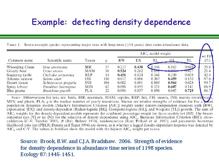
Example: detecting density dependence Source: Brook, B. W. and C. J. A. Bradshaw. 2006. Strength of evidence for density dependence in abundance time series of 1198 species. Ecology 87: 1445 -1451.

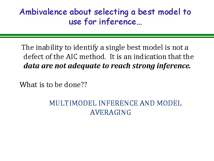
Ambivalence about selecting a best model to use for inference… The inability to identify a single best model is not a defect of the AIC method. It is an indication that the data are not adequate to reach strong inference. What is to be done? ? MULTIMODEL INFERENCE AND MODEL AVERAGING

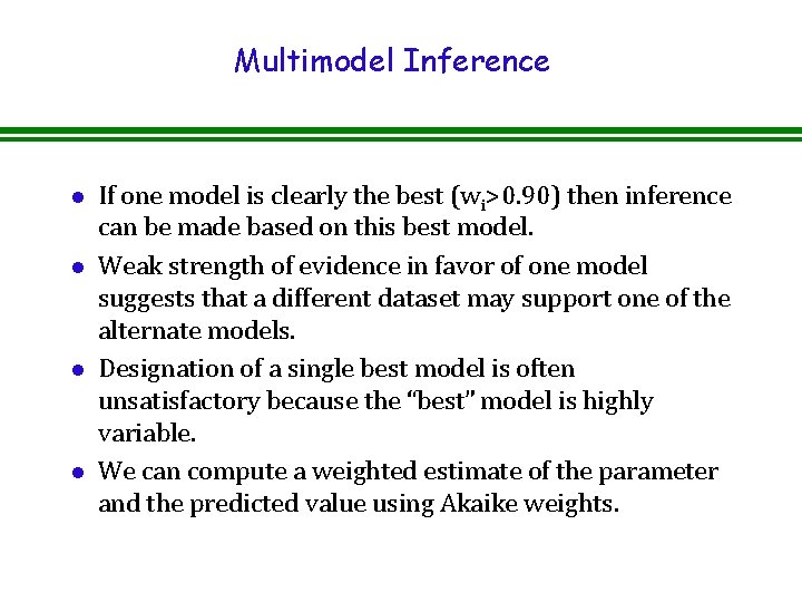
Multimodel Inference l l If one model is clearly the best (wi>0. 90) then inference can be made based on this best model. Weak strength of evidence in favor of one model suggests that a different dataset may support one of the alternate models. Designation of a single best model is often unsatisfactory because the “best” model is highly variable. We can compute a weighted estimate of the parameter and the predicted value using Akaike weights.

Akaike Weights and Multimodel Inference l l Estimate parameter values for the models with at least some measurable support. Estimate weighted average of parameters across those models. Only applicable to linear models. For non-linear models, we can generate weighted averages of the predicted response value for given values of the predictor variables.

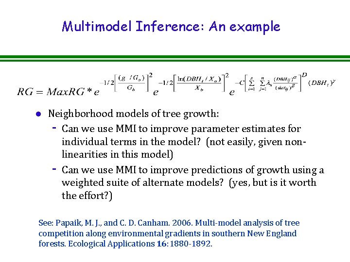
Multimodel Inference: An example l Neighborhood models of tree growth: - Can we use MMI to improve parameter estimates for individual terms in the model? (not easily, given nonlinearities in this model) - Can we use MMI to improve predictions of growth using a weighted suite of alternate models? (yes, but is it worth the effort? ) See: Papaik, M. J. , and C. D. Canham. 2006. Multi-model analysis of tree competition along environmental gradients in southern New England forests. Ecological Applications 16: 1880 -1892.

Summary: Steps in Model Selection l Develop candidate models based on biological knowledge. l Take observations (data) relevant to predictions of the model. l Use data to obtain MLE of parameters of the alternate models. l Evaluate strength of evidence for alternate models using AIC and Akaike weights. l …Multimodel Inference? Do you agree with Burnham and Anderson that MMI is generally preferable to “best-model inference”?

Bias and Uncertainty in Model Selection l Model Selection Bias: Chance inclusion of meaningless variables in a model will produce a biased underestimate of the variance, and a corresponding exaggeration of the precision of the model (the problem with “fishing expeditions”) l Model Selection Uncertainty: The fact that we are using data (with uncertainty) to both estimate parameters and to select the best model necessarily introduces uncertainty into the model selection process See discussion on pages 43 -47 of Burnham and Anderson

The brave new world… l Science is the development of simplified models as explanations (approximations) of reality… l The “quality” of the explanation (the model) will be a balance of many factors (both quantitative and qualitative)