gradient Descent py def gradient Descentx y theta

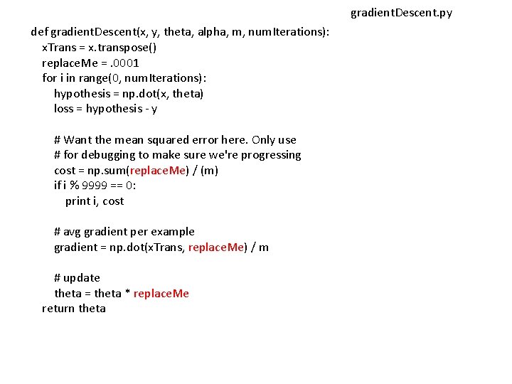
gradient. Descent. py def gradient. Descent(x, y, theta, alpha, m, num. Iterations): x. Trans = x. transpose() replace. Me =. 0001 for i in range(0, num. Iterations): hypothesis = np. dot(x, theta) loss = hypothesis - y # Want the mean squared error here. Only use # for debugging to make sure we're progressing cost = np. sum(replace. Me) / (m) if i % 9999 == 0: print i, cost # avg gradient per example gradient = np. dot(x. Trans, replace. Me) / m # update theta = theta * replace. Me return theta

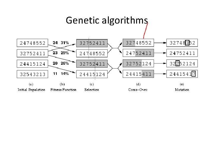
Genetic algorithms

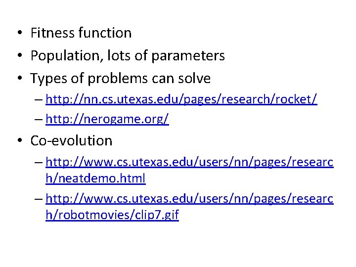
• Fitness function • Population, lots of parameters • Types of problems can solve – http: //nn. cs. utexas. edu/pages/research/rocket/ – http: //nerogame. org/ • Co-evolution – http: //www. cs. utexas. edu/users/nn/pages/researc h/neatdemo. html – http: //www. cs. utexas. edu/users/nn/pages/researc h/robotmovies/clip 7. gif

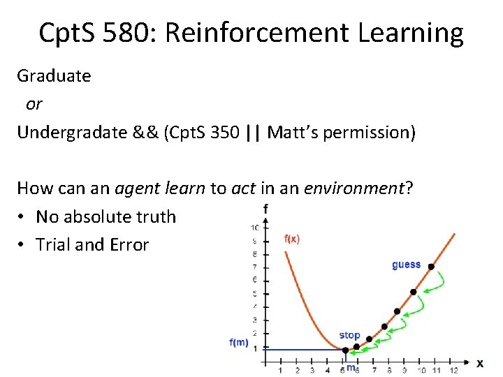
Cpt. S 580: Reinforcement Learning Graduate or Undergradate && (Cpt. S 350 || Matt’s permission) How can an agent learn to act in an environment? • No absolute truth • Trial and Error

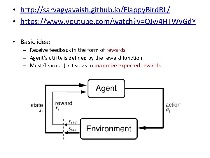
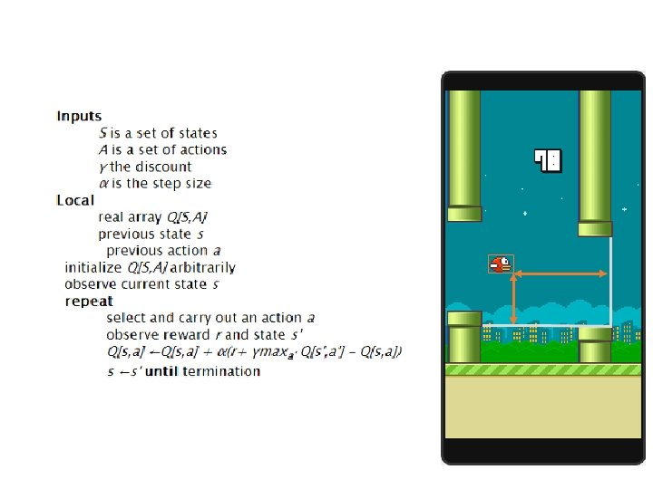
• http: //sarvagyavaish. github. io/Flappy. Bird. RL/ • https: //www. youtube. com/watch? v=OJw 4 HTWv. Gd. Y • Basic idea: – Receive feedback in the form of rewards – Agent’s utility is defined by the reward function – Must (learn to) act so as to maximize expected rewards

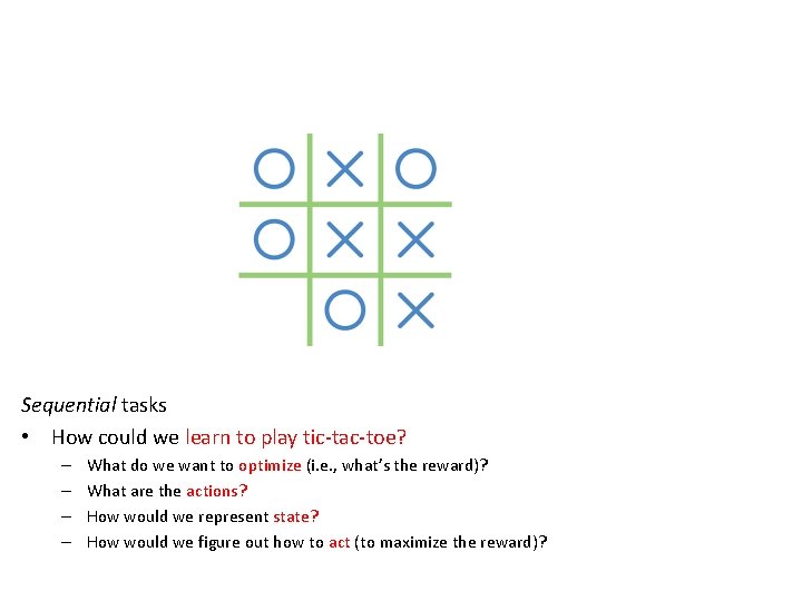
Sequential tasks • How could we learn to play tic-tac-toe? – – What do we want to optimize (i. e. , what’s the reward)? What are the actions? How would we represent state? How would we figure out how to act (to maximize the reward)?

Reinforcement Learning (RL) • RL algorithms attempt to find a policy – maximizing cumulative reward for the agent – over the course of the problem • Typically represented by a Markov Decision Process • RL differs from supervised learning: – correct input/output pairs are never presented – sub-optimal actions never explicitly corrected

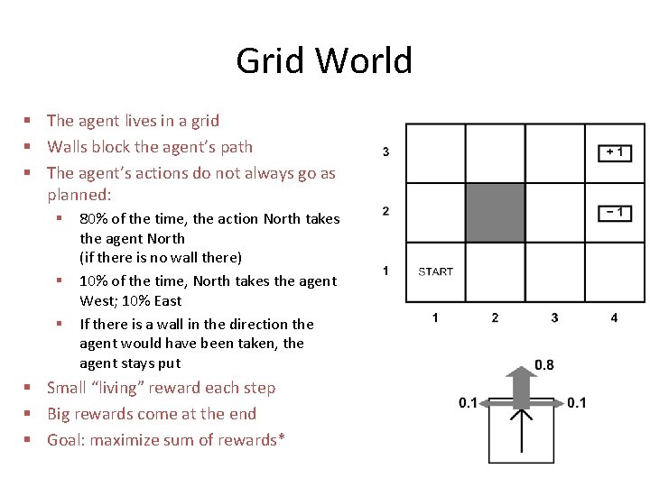
Grid World § The agent lives in a grid § Walls block the agent’s path § The agent’s actions do not always go as planned: § § § 80% of the time, the action North takes the agent North (if there is no wall there) 10% of the time, North takes the agent West; 10% East If there is a wall in the direction the agent would have been taken, the agent stays put § Small “living” reward each step § Big rewards come at the end § Goal: maximize sum of rewards*

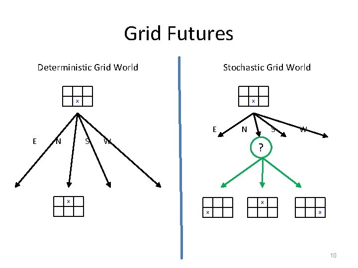
Grid Futures Deterministic Grid World Stochastic Grid World X X E E N S W ? X X 10

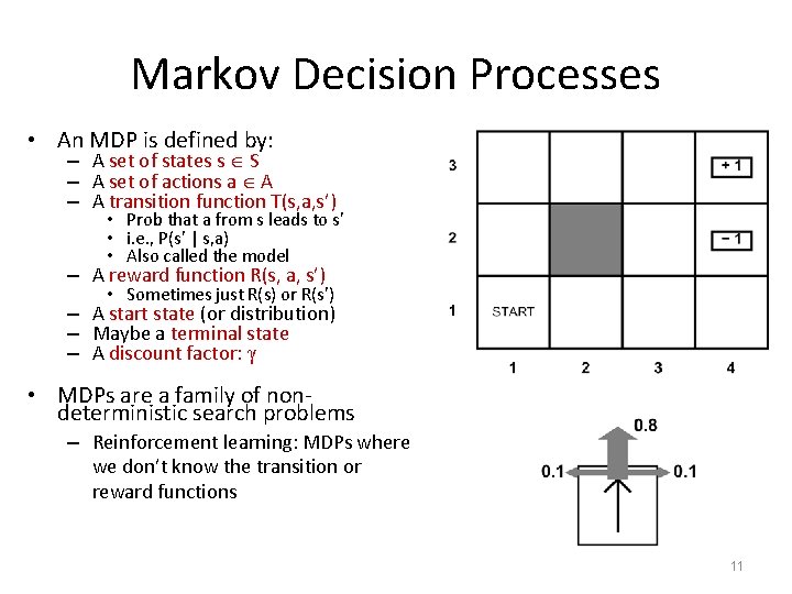
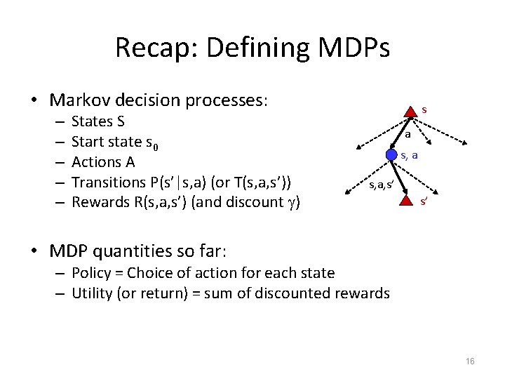
Markov Decision Processes • An MDP is defined by: – A set of states s S – A set of actions a A – A transition function T(s, a, s’) • Prob that a from s leads to s’ • i. e. , P(s’ | s, a) • Also called the model – A reward function R(s, a, s’) • Sometimes just R(s) or R(s’) – A start state (or distribution) – Maybe a terminal state – A discount factor: γ • MDPs are a family of nondeterministic search problems – Reinforcement learning: MDPs where we don’t know the transition or reward functions 11

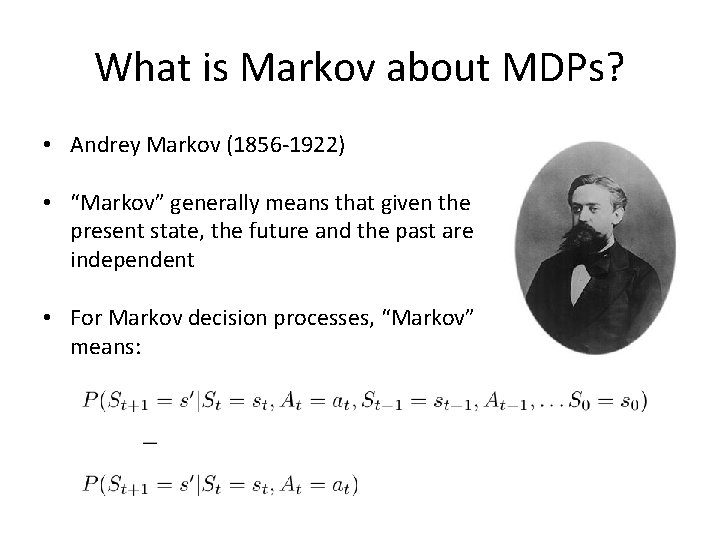
What is Markov about MDPs? • Andrey Markov (1856 -1922) • “Markov” generally means that given the present state, the future and the past are independent • For Markov decision processes, “Markov” means:

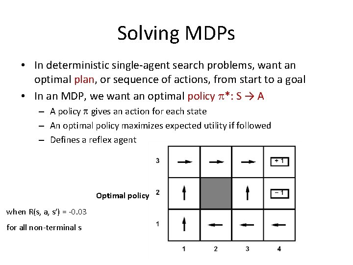
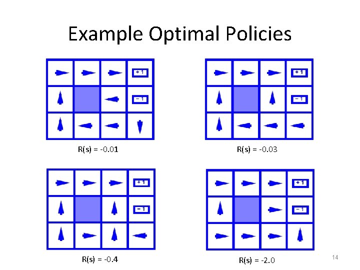
Solving MDPs • In deterministic single-agent search problems, want an optimal plan, or sequence of actions, from start to a goal • In an MDP, we want an optimal policy *: S → A – A policy gives an action for each state – An optimal policy maximizes expected utility if followed – Defines a reflex agent Optimal policy when R(s, a, s’) = -0. 03 for all non-terminal s

Example Optimal Policies R(s) = -0. 01 R(s) = -0. 03 R(s) = -0. 4 R(s) = -2. 0 14

Recap: Defining MDPs • Markov decision processes: – – – States S Start state s 0 Actions A Transitions P(s’|s, a) (or T(s, a, s’)) Rewards R(s, a, s’) (and discount ) s a s, a, s’ s’ • MDP quantities so far: – Policy = Choice of action for each state – Utility (or return) = sum of discounted rewards 16

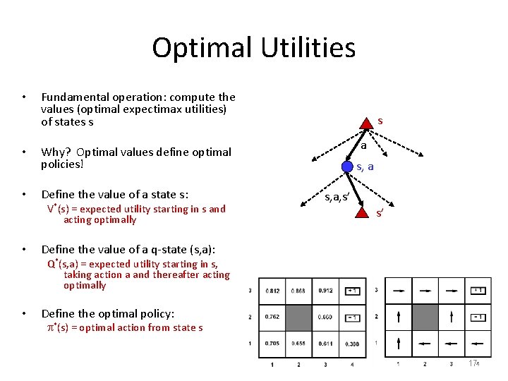
Optimal Utilities • Fundamental operation: compute the values (optimal expectimax utilities) of states s • Why? Optimal values define optimal policies! • Define the value of a state s: V*(s) = expected utility starting in s and acting optimally • s a s, a, s’ s’ Define the value of a q-state (s, a): Q*(s, a) = expected utility starting in s, taking action a and thereafter acting optimally • Define the optimal policy: *(s) = optimal action from state s 17

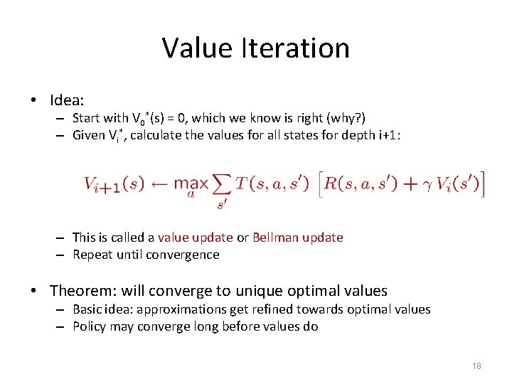
Value Iteration • Idea: – Start with V 0*(s) = 0, which we know is right (why? ) – Given Vi*, calculate the values for all states for depth i+1: – This is called a value update or Bellman update – Repeat until convergence • Theorem: will converge to unique optimal values – Basic idea: approximations get refined towards optimal values – Policy may converge long before values do 18

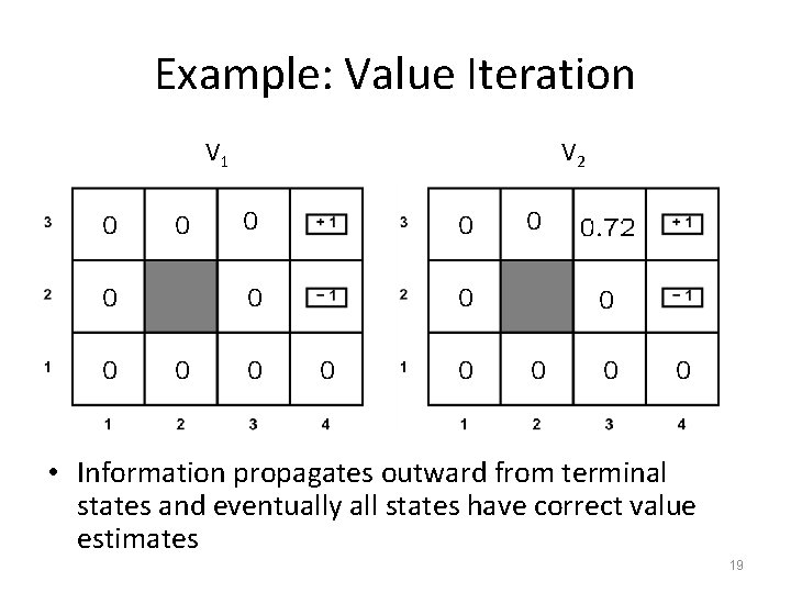
Example: Value Iteration V 1 V 2 • Information propagates outward from terminal states and eventually all states have correct value estimates 19

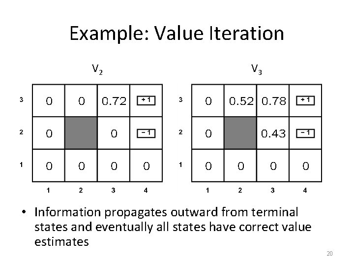
Example: Value Iteration V 2 V 3 • Information propagates outward from terminal states and eventually all states have correct value estimates 20

Discounted Rewards • Rewards in the future are worth less than an immediate reward – Because of uncertainty: who knows if/when you’re going to get to that reward state

Discounted Rewards • Discount factor ϒ (often. 9 -1. 0) • Assume a reward years in the future is only worth of the value of immediate reward • For each state, calculate a utility value equal to the Sum of Future Discounted Rewards

Reinforcement Learning • Reinforcement learning: – Still assume an MDP: • • • A set of states s S A set of actions (per state) A A model T(s, a, s’) A reward function R(s, a, s’) A discount factor γ (could be 1) – Still looking for a policy (s) – New twist: don’t know T or R • i. e. don’t know which states are good or what the actions do • Must actually try actions and states out to learn 23

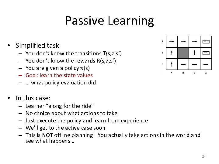
Passive Learning • Simplified task – – – You don’t know the transitions T(s, a, s’) You don’t know the rewards R(s, a, s’) You are given a policy (s) Goal: learn the state values … what policy evaluation did • In this case: – – – Learner “along for the ride” No choice about what actions to take Just execute the policy and learn from experience We’ll get to the active case soon This is NOT offline planning! You actually take actions in the world and see what happens… 24

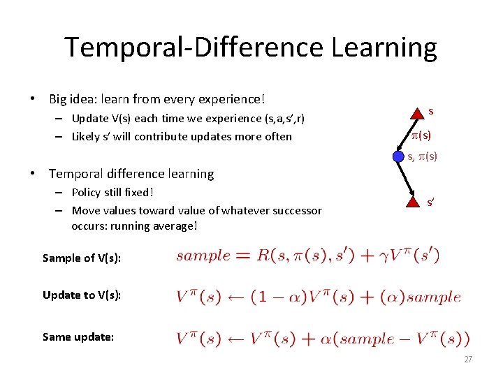
Temporal-Difference Learning • Big idea: learn from every experience! – Update V(s) each time we experience (s, a, s’, r) – Likely s’ will contribute updates more often s (s) s, (s) • Temporal difference learning – Policy still fixed! – Move values toward value of whatever successor occurs: running average! s’ Sample of V(s): Update to V(s): Same update: 27

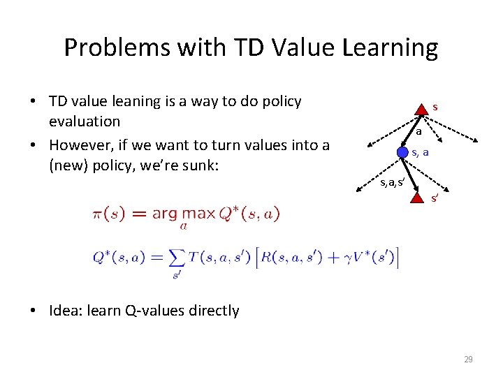
Problems with TD Value Learning • TD value leaning is a way to do policy evaluation • However, if we want to turn values into a (new) policy, we’re sunk: s a s, a, s’ s’ • Idea: learn Q-values directly 29

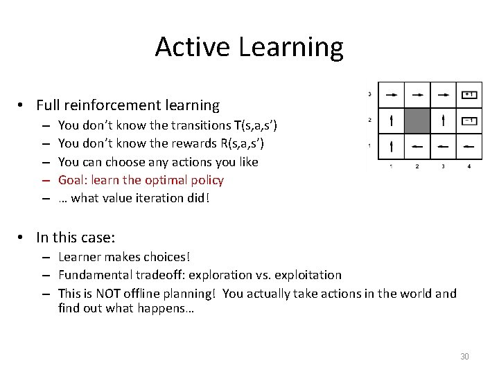
Active Learning • Full reinforcement learning – – – You don’t know the transitions T(s, a, s’) You don’t know the rewards R(s, a, s’) You can choose any actions you like Goal: learn the optimal policy … what value iteration did! • In this case: – Learner makes choices! – Fundamental tradeoff: exploration vs. exploitation – This is NOT offline planning! You actually take actions in the world and find out what happens… 30

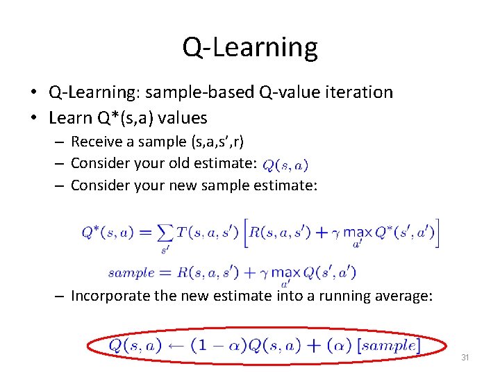
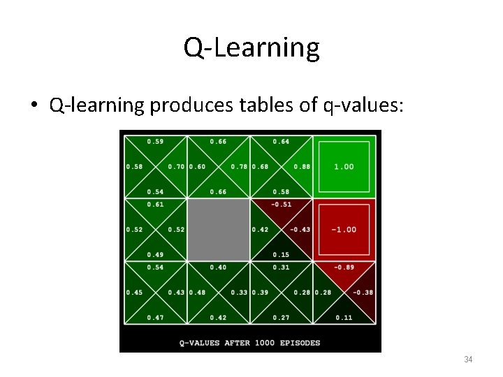
Q-Learning • Q-Learning: sample-based Q-value iteration • Learn Q*(s, a) values – Receive a sample (s, a, s’, r) – Consider your old estimate: – Consider your new sample estimate: – Incorporate the new estimate into a running average: 31

Q-Learning • Q-learning produces tables of q-values: 34

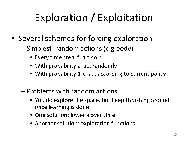
Exploration / Exploitation • Several schemes forcing exploration – Simplest: random actions ( greedy) • Every time step, flip a coin • With probability , act randomly • With probability 1 - , act according to current policy – Problems with random actions? • You do explore the space, but keep thrashing around once learning is done • One solution: lower over time • Another solution: exploration functions 35

Q-Learning • In realistic situations, we cannot possibly learn about every single state! – Too many states to visit them all in training – Too many states to hold the q-tables in memory • Instead, we want to generalize: – Learn about some small number of training states from experience – Generalize that experience to new, similar states – This is a fundamental idea in machine learning, and we’ll see it over and over again 37

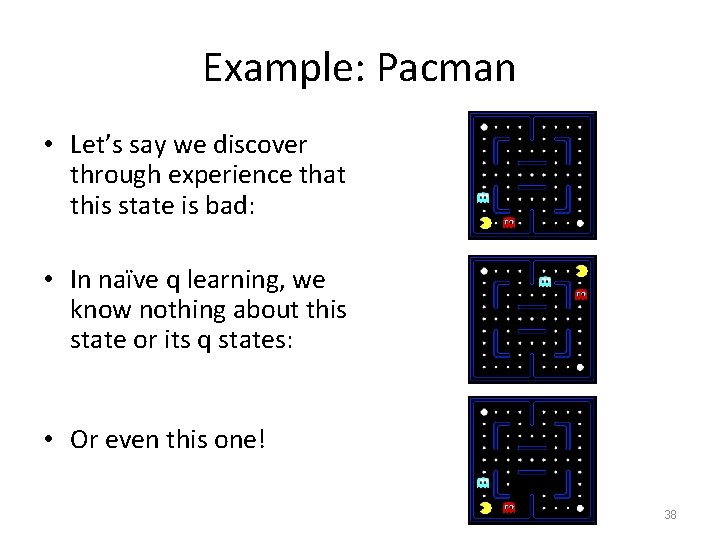
Example: Pacman • Let’s say we discover through experience that this state is bad: • In naïve q learning, we know nothing about this state or its q states: • Or even this one! 38

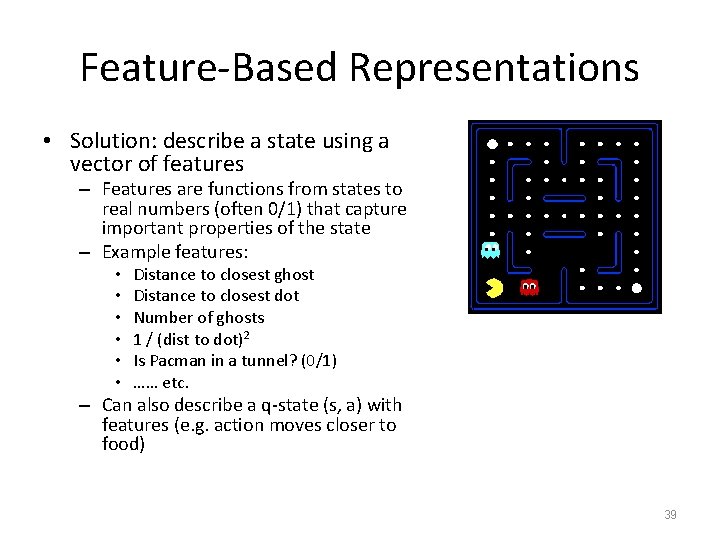
Feature-Based Representations • Solution: describe a state using a vector of features – Features are functions from states to real numbers (often 0/1) that capture important properties of the state – Example features: • • • Distance to closest ghost Distance to closest dot Number of ghosts 1 / (dist to dot)2 Is Pacman in a tunnel? (0/1) …… etc. – Can also describe a q-state (s, a) with features (e. g. action moves closer to food) 39

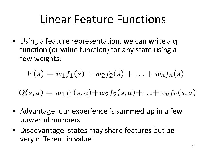
Linear Feature Functions • Using a feature representation, we can write a q function (or value function) for any state using a few weights: • Advantage: our experience is summed up in a few powerful numbers • Disadvantage: states may share features but be very different in value! 40

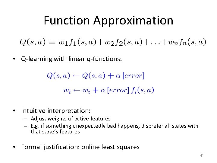
Function Approximation • Q-learning with linear q-functions: • Intuitive interpretation: – Adjust weights of active features – E. g. if something unexpectedly bad happens, disprefer all states with that state’s features • Formal justification: online least squares 41