Statistical Genomics Lecture 4 Statistical inference Zhiwu Zhang

Statistical Genomics Lecture 4: Statistical inference Zhiwu Zhang Washington State University

Outline X 2 test on contingency table Empirical null distribution X 2 test on variance t test Hypothesis test two types of error Power

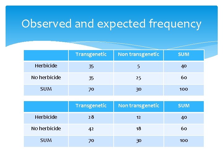
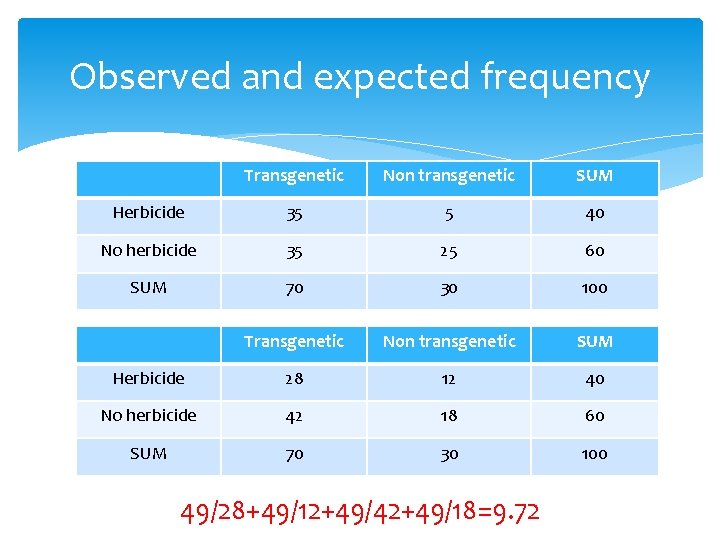
Observed and expected frequency Transgenetic Non transgenetic SUM Herbicide 35 5 40 No herbicide 35 25 60 SUM 70 30 100 Transgenetic Non transgenetic SUM Herbicide 28 12 40 No herbicide 42 18 60 SUM 70 30 100

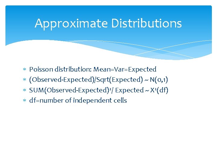
Approximate Distributions Poisson distribution: Mean=Var=Expected (Observed-Expected)/Sqrt(Expected) ~ N(0, 1) SUM(Observed-Expected)2/ Expected ~ X 2(df) df=number of independent cells

Observed and expected frequency Transgenetic Non transgenetic SUM Herbicide 35 5 40 No herbicide 35 25 60 SUM 70 30 100 Transgenetic Non transgenetic SUM Herbicide 28 12 40 No herbicide 42 18 60 SUM 70 30 100 49/28+49/12+49/42+49/18=9. 72

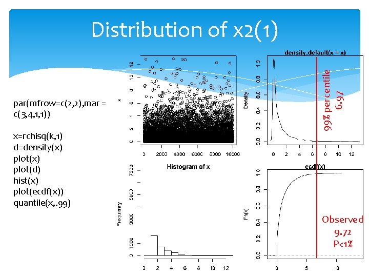
par(mfrow=c(2, 2), mar = c(3, 4, 1, 1)) x=rchisq(k, 1) d=density(x) plot(d) hist(x) plot(ecdf(x)) quantile(x, . 99) 99% percentile 6. 97 Distribution of x 2(1) Observed 9. 72 P<1%

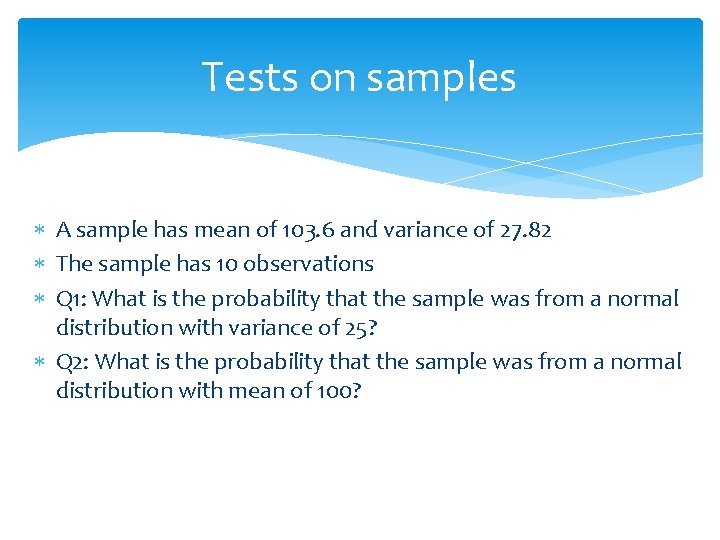
Tests on samples A sample has mean of 103. 6 and variance of 27. 82 The sample has 10 observations Q 1: What is the probability that the sample was from a normal distribution with variance of 25? Q 2: What is the probability that the sample was from a normal distribution with mean of 100?

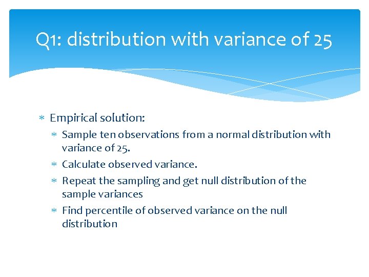
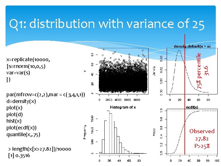
Q 1: distribution with variance of 25 Empirical solution: Sample ten observations from a normal distribution with variance of 25. Calculate observed variance. Repeat the sampling and get null distribution of the sample variances Find percentile of observed variance on the null distribution

x=replicate(10000, {s=rnorm(10, 0, 5) var=var(s) }) par(mfrow=c(2, 2), mar = c(3, 4, 1, 1)) d=density(x) plot(d) hist(x) plot(ecdf(x)) quantile(x, . 75) > length(x[x>27. 82])/10000 [1] 0. 3516 75% percentile 31. 6 Q 1: distribution with variance of 25 Observed 27. 82 P>25%

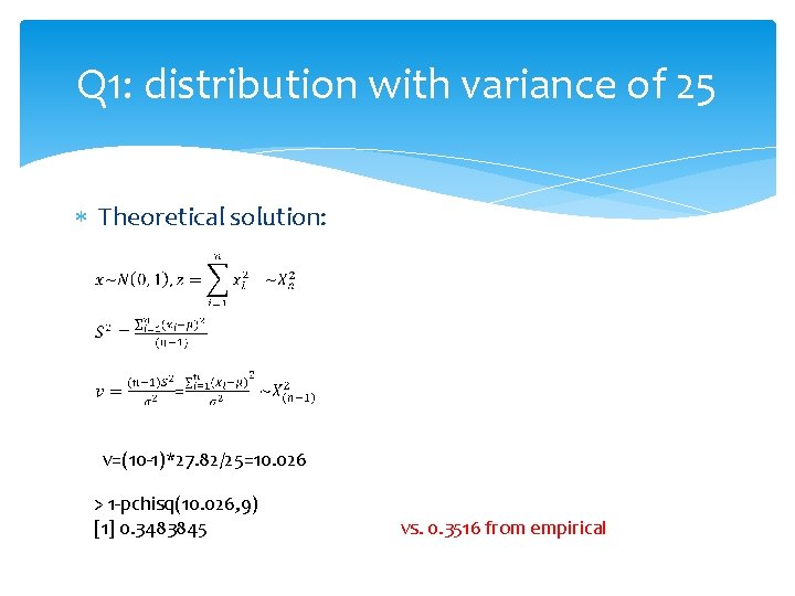
Q 1: distribution with variance of 25 Theoretical solution: v=(10 -1)*27. 82/25=10. 026 > 1 -pchisq(10. 026, 9) [1] 0. 3483845 vs. 0. 3516 from empirical

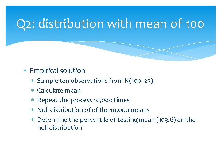
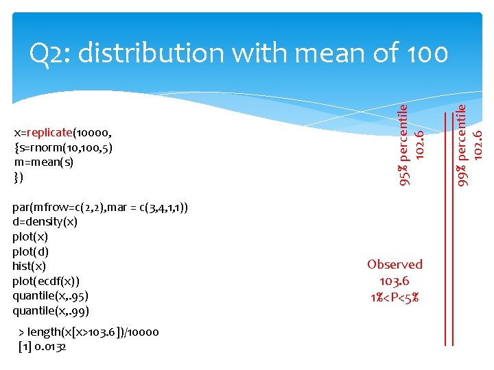
Q 2: distribution with mean of 100 Empirical solution Sample ten observations from N(100, 25) Calculate mean Repeat the process 10, 000 times Null distribution of of the 10, 000 means Determine the percentile of testing mean (103. 6) on the null distribution

par(mfrow=c(2, 2), mar = c(3, 4, 1, 1)) d=density(x) plot(d) hist(x) plot(ecdf(x)) quantile(x, . 95) quantile(x, . 99) > length(x[x>103. 6])/10000 [1] 0. 0132 Observed 103. 6 1%<P<5% 99% percentile 102. 6 x=replicate(10000, {s=rnorm(10, 100, 5) m=mean(s) }) 95% percentile 102. 6 Q 2: distribution with mean of 100

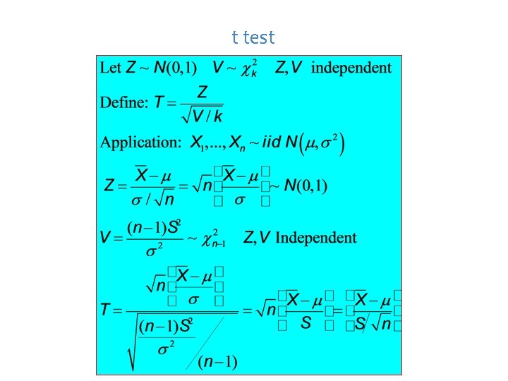
t test

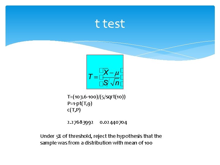
t test T=(103. 6 -100)/(5/sqrt(10)) P=1 -pt(T, 9) c(T, P) 2. 27683992 0. 02440704 Under 5% of threshold, reject the hypothesis that the sample was from a distribution with mean of 100

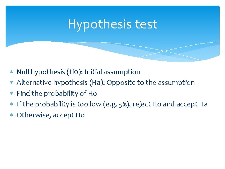
Hypothesis test Null hypothesis (H 0): Initial assumption Alternative hypothesis (Ha): Opposite to the assumption Find the probability of H 0 If the probability is too low (e. g. 5%), reject Ho and accept Ha Otherwise, accept Ho

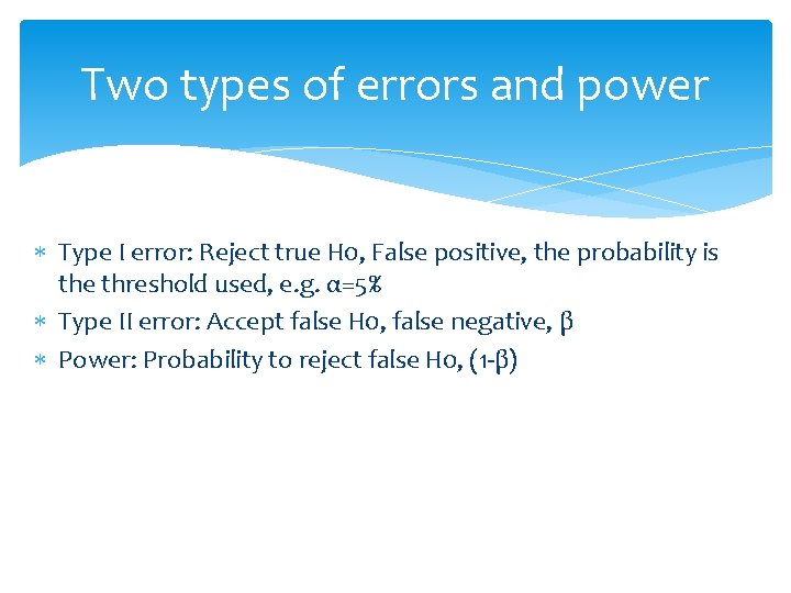
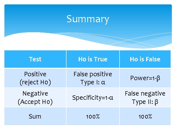
Two types of errors and power Type I error: Reject true H 0, False positive, the probability is the threshold used, e. g. α=5% Type II error: Accept false H 0, false negative, β Power: Probability to reject false H 0, (1 -β)

Summary Test H 0 is True Ho is False Positive (reject H 0) False positive Type I: α Power=1 -β Negative (Accept H 0) Specificity=1 -α False negative Type II: β Sum 100%

Highlight X 2 test on contingency table Empirical null distribution X 2 test on variance t test Hypothesis test two types of error Power