Simple Harmonic Motion AH Physics QW Mr Stewart


- Slides: 22

Simple Harmonic Motion AH Physics Q&W Mr Stewart

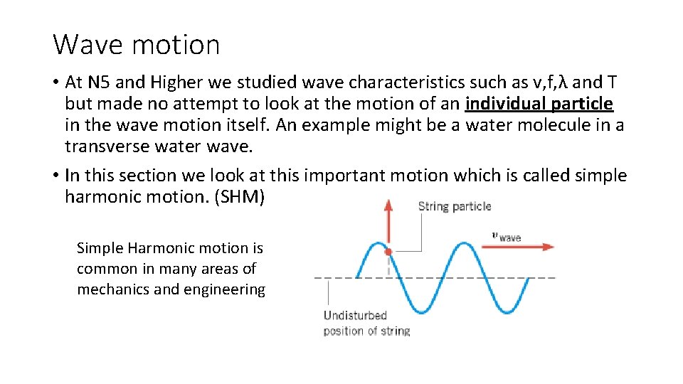
Wave motion • At N 5 and Higher we studied wave characteristics such as v, f, λ and T but made no attempt to look at the motion of an individual particle in the wave motion itself. An example might be a water molecule in a transverse water wave. • In this section we look at this important motion which is called simple harmonic motion. (SHM) Simple Harmonic motion is common in many areas of mechanics and engineering

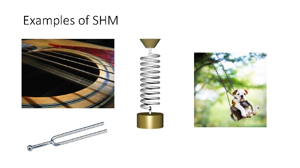
Examples of SHM

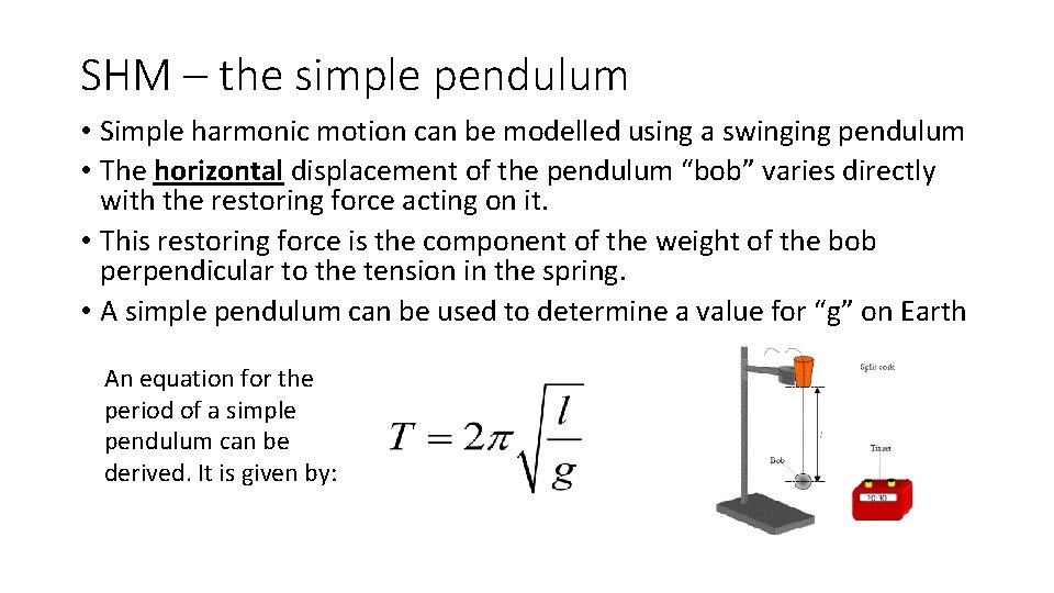
SHM – the simple pendulum • Simple harmonic motion can be modelled using a swinging pendulum • The horizontal displacement of the pendulum “bob” varies directly with the restoring force acting on it. • This restoring force is the component of the weight of the bob perpendicular to the tension in the spring. • A simple pendulum can be used to determine a value for “g” on Earth An equation for the period of a simple pendulum can be derived. It is given by:

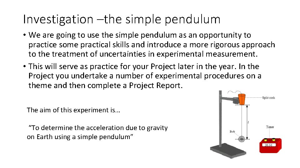
Investigation –the simple pendulum • We are going to use the simple pendulum as an opportunity to practice some practical skills and introduce a more rigorous approach to the treatment of uncertainties in experimental measurement. • This will serve as practice for your Project later in the year. In the Project you undertake a number of experimental procedures on a theme and then complete a Project Report. The aim of this experiment is… “To determine the acceleration due to gravity on Earth using a simple pendulum”

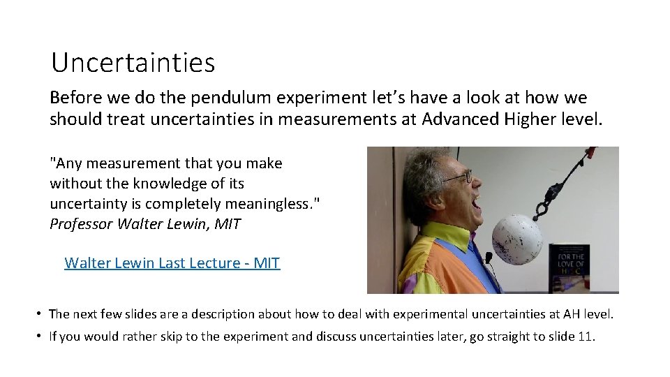
Uncertainties Before we do the pendulum experiment let’s have a look at how we should treat uncertainties in measurements at Advanced Higher level. "Any measurement that you make without the knowledge of its uncertainty is completely meaningless. " Professor Walter Lewin, MIT Walter Lewin Last Lecture - MIT • The next few slides are a description about how to deal with experimental uncertainties at AH level. • If you would rather skip to the experiment and discuss uncertainties later, go straight to slide 11.

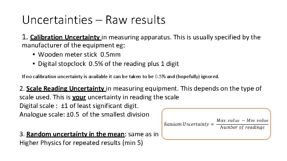
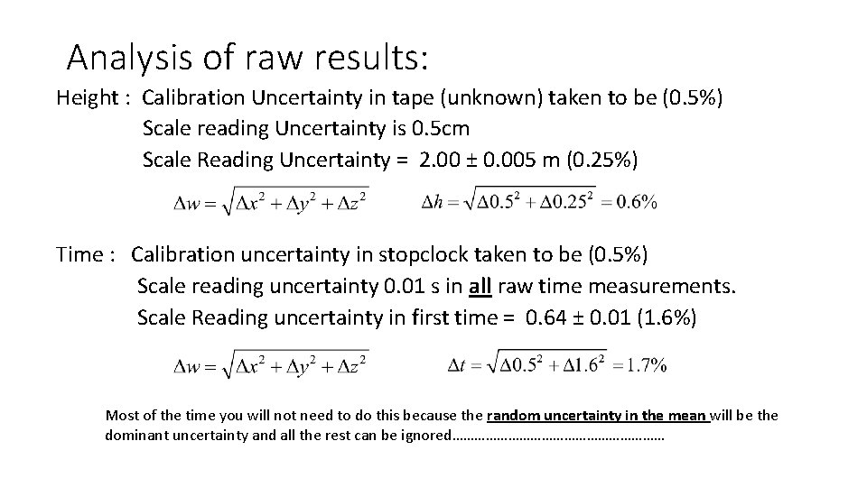
Uncertainties – Raw results 1. Calibration Uncertainty in measuring apparatus. This is usually specified by the manufacturer of the equipment eg: • Wooden meter stick 0. 5 mm • Digital stopclock 0. 5% of the reading plus 1 digit If no calibration uncertainty is available it can be taken to be 0. 5% and (hopefully) ignored. 2. Scale Reading Uncertainty in measuring equipment. This depends on the type of scale used. This is your uncertainty in reading the scale Digital scale : ± 1 of least significant digit. Analogue scale: ± 0. 5 of the smallest division 3. Random uncertainty in the mean: same as in Higher Physics for repeated results (min 5)

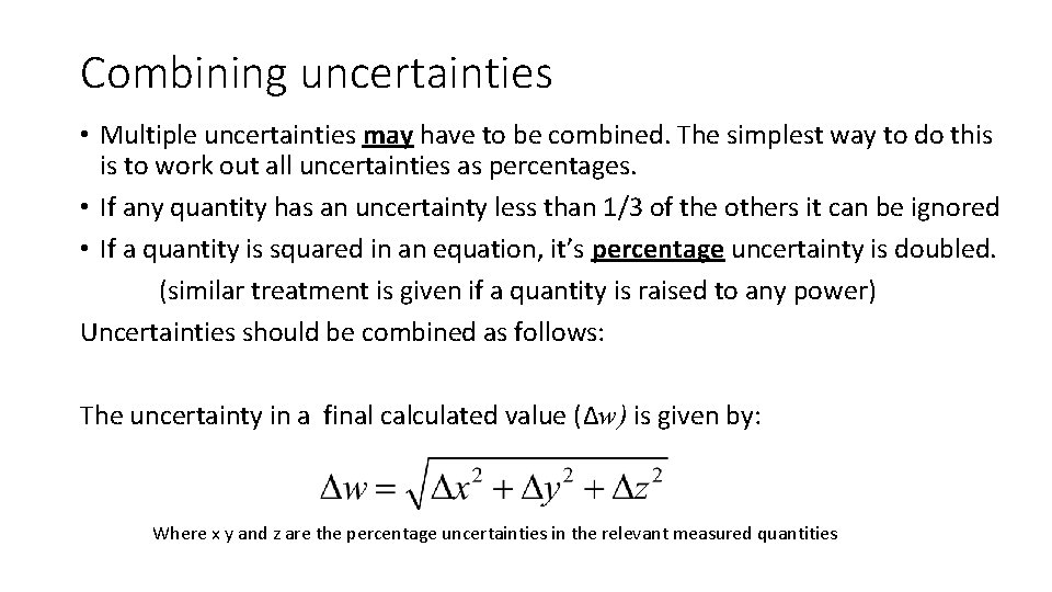
Combining uncertainties • Multiple uncertainties may have to be combined. The simplest way to do this is to work out all uncertainties as percentages. • If any quantity has an uncertainty less than 1/3 of the others it can be ignored • If a quantity is squared in an equation, it’s percentage uncertainty is doubled. (similar treatment is given if a quantity is raised to any power) Uncertainties should be combined as follows: The uncertainty in a final calculated value (Δw) is given by: Where x y and z are the percentage uncertainties in the relevant measured quantities

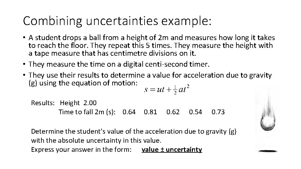
Combining uncertainties example: • A student drops a ball from a height of 2 m and measures how long it takes to reach the floor. They repeat this 5 times. They measure the height with a tape measure that has centimetre divisions on it. • They measure the time on a digital centi-second timer. • They use their results to determine a value for acceleration due to gravity (g) using the equation of motion: Results: Height 2. 00 Time to fall 2 m (s): 0. 64 0. 81 0. 62 0. 54 0. 73 Determine the student’s value of the acceleration due to gravity (g) with the absolute uncertainty in this value. Express your answer in the form: value ± uncertainty

Analysis of raw results: Height : Calibration Uncertainty in tape (unknown) taken to be (0. 5%) Scale reading Uncertainty is 0. 5 cm Scale Reading Uncertainty = 2. 00 ± 0. 005 m (0. 25%) Time : Calibration uncertainty in stopclock taken to be (0. 5%) Scale reading uncertainty 0. 01 s in all raw time measurements. Scale Reading uncertainty in first time = 0. 64 ± 0. 01 (1. 6%) Most of the time you will not need to do this because the random uncertainty in the mean will be the dominant uncertainty and all the rest can be ignored…………………………

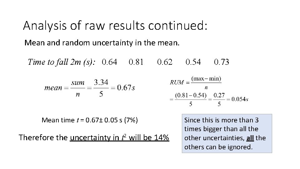
Analysis of raw results continued: Mean and random uncertainty in the mean. Time to fall 2 m (s): 0. 64 0. 81 0. 62 Mean time t = 0. 67± 0. 05 s (7%) Therefore the uncertainty in t 2 will be 14% 0. 54 0. 73 Since this is more than 3 times bigger than all the other uncertainties, all the others can be ignored.

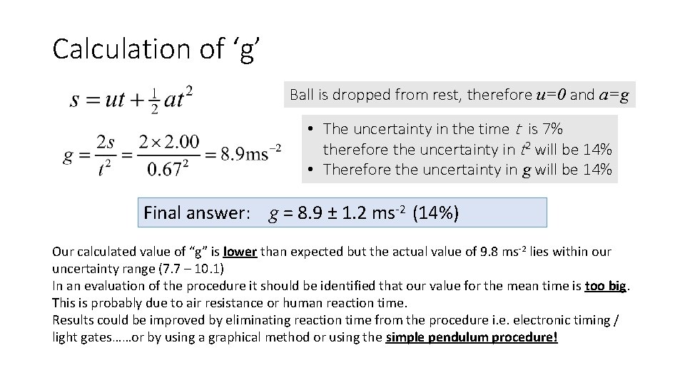
Calculation of ‘g’ Ball is dropped from rest, therefore u=0 and a=g • The uncertainty in the time t is 7% therefore the uncertainty in t 2 will be 14% • Therefore the uncertainty in g will be 14% Final answer: g = 8. 9 ± 1. 2 ms-2 (14%) Our calculated value of “g” is lower than expected but the actual value of 9. 8 ms-2 lies within our uncertainty range (7. 7 – 10. 1) In an evaluation of the procedure it should be identified that our value for the mean time is too big. This is probably due to air resistance or human reaction time. Results could be improved by eliminating reaction time from the procedure i. e. electronic timing / light gates……or by using a graphical method or using the simple pendulum procedure!

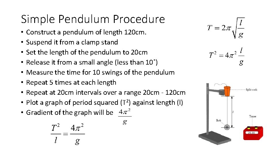
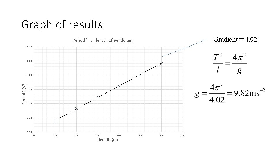
Simple Pendulum Procedure • • • Construct a pendulum of length 120 cm. Suspend it from a clamp stand Set the length of the pendulum to 20 cm Release it from a small angle (less than 10˚) Measure the time for 10 swings of the pendulum Repeat 5 times at each length Repeat at 20 cm intervals over a range 20 cm - 120 cm Plot a graph of period squared (T 2) against length (l) Gradient of the graph will be

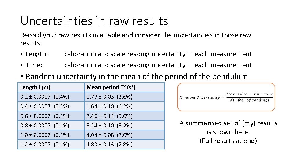
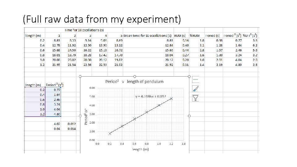
Uncertainties in raw results Record your raw results in a table and consider the uncertainties in those raw results: • Length: calibration and scale reading uncertainty in each measurement • Time: calibration and scale reading uncertainty in each measurement • Random uncertainty in the mean of the period of the pendulum Length l (m) Mean period T 2 (s 2) 0. 2 ± 0. 0007 (0. 4%) 0. 77 ± 0. 03 (3. 6%) 0. 4 ± 0. 0007 (0. 2%) 1. 64 ± 0. 10 (6. 2%) 0. 6 ± 0. 0007 (0. 1%) 2. 46 ± 0. 14 (5. 6%) 0. 8 ± 0. 0007 (0. 1%) 3. 24 ± 0. 10 (3. 2%) 1. 0 ± 0. 0007 (0. 1%) 4. 04 ± 0. 08 (2. 0%) 1. 2 ± 0. 0007 (0. 1%) 4. 80 ± 0. 13 (2. 8%) A summarised set of (my) results is shown here. (Full results at end)

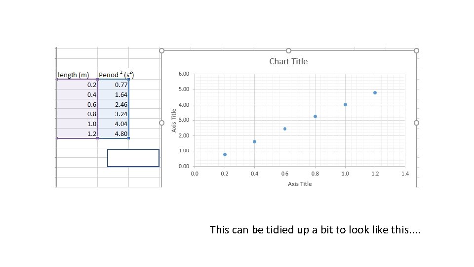
Using a graphical method • Use Excel – it will make your life so much easier! • Enter your appropriate raw results on a spreadsheet then insert an x y scatter graph. • Get excel to draw the best fit line and display the equation of the line on the graph • This will show you the gradient and the y-intercept. • The y-intercept will show you if there is a systematic uncertainty in your procedure. • The uncertainty in the gradient can be determined using the LINEST function (see separate handout)

This can be tidied up a bit to look like this. .

Graph of results Gradient = 4. 02 Period 2 v length of pendulum 6. 00 5. 00 Period 2 (s 2) 4. 00 3. 00 2. 00 1. 00 0. 2 0. 4 0. 6 0. 8 length (m) 1. 0 1. 2 1. 4

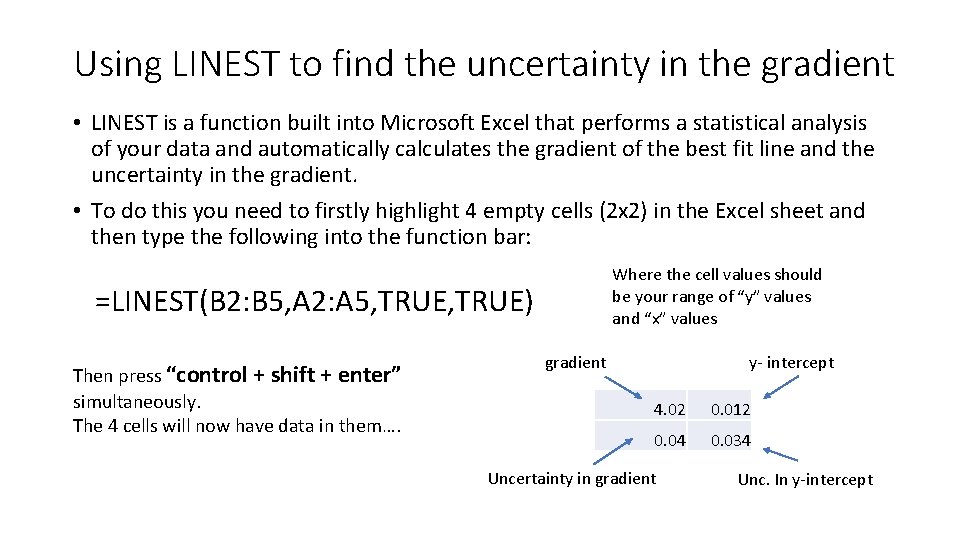
Using LINEST to find the uncertainty in the gradient • LINEST is a function built into Microsoft Excel that performs a statistical analysis of your data and automatically calculates the gradient of the best fit line and the uncertainty in the gradient. • To do this you need to firstly highlight 4 empty cells (2 x 2) in the Excel sheet and then type the following into the function bar: Where the cell values should be your range of “y” values and “x” values =LINEST(B 2: B 5, A 2: A 5, TRUE) Then press “control + shift + enter” simultaneously. The 4 cells will now have data in them…. y- intercept gradient 4. 02 0. 012 0. 04 0. 034 Uncertainty in gradient Unc. In y-intercept

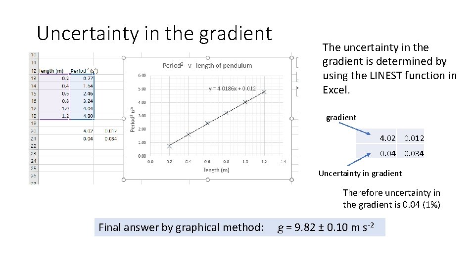
Uncertainty in the gradient The uncertainty in the gradient is determined by using the LINEST function in Excel. gradient 4. 02 0. 012 0. 04 0. 034 Uncertainty in gradient Therefore uncertainty in the gradient is 0. 04 (1%) Final answer by graphical method: g = 9. 82 ± 0. 10 m s-2

Systematic uncertainty • Our graph doesn’t go through the origin. • From the LINEST function we can see there is a y-intercept of 0. 012. • This implies that our period or length measurements are all out by the same amount (due to human reaction times? – very unlikely) • It is more likely that we have a systematic uncertainty in our length measurement: We are not measuring the centre of the bob from the point of suspension correctly. We have measured too short (by 3 mm) • A graph that doesn’t go through the origin points to a systematic uncertainty. (Note a systematic uncertainty doesn’t affect the gradient, this is why a graphical method is better. )

Report Write up a report on the experiment using the “instructions for candidates” to guide you through the format of the report. Basically: • Title • Aim • Apparatus • Uncertainties • Conclusion • Evaluation • Procedure (written in impersonal past tense) • Results There is a sample report available for you to use as a guide. Email your report to your teacher when finished!

(Full raw data from my experiment)