Sequenziamento metodo di Sanger con dd NTP Sequenziamento

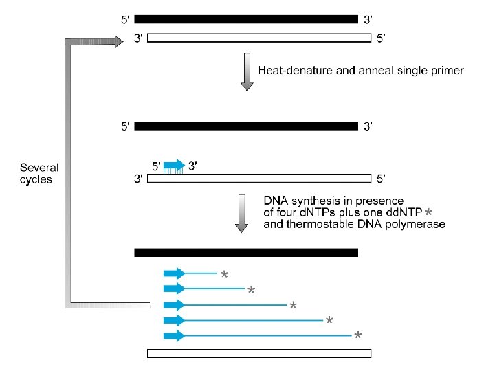
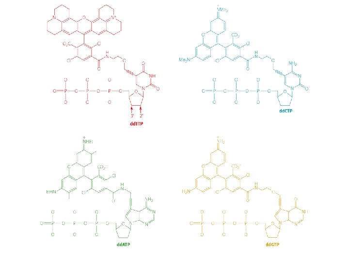
Sequenziamento: metodo di Sanger con dd. NTP

Sequenziamento con dideossonucleotidi

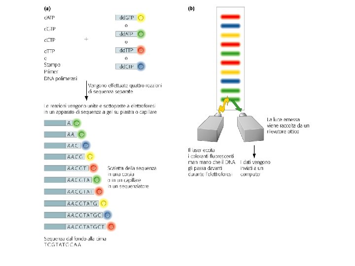
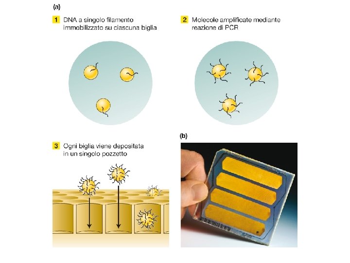
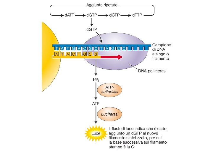
Sequenziamento automatizzato del DNA

Clonaggio: Inserto Vettore + Ligazione

Trattamento del vettore con fosfatasi AATTC G G CTTAA p. AATTC G G CTTAAp Eco. RI GAATTC CTTAAG C TT p. G AA A G TTA C DNA ligasi G CT p. AA TA TT A C G fosfatasi

Vettori plasmidici (p. BR 322)

Vettori plasmidici (p. UC 18)

• Ceppo di E. coli Lac Z mutante • Vettore p. UC Lac. Z parziale • Ceppo di E. coli Lac Z mutante • Vettore Lac. Z interrotto dal clonaggio Complementano Non c’è complementazione β-galattosidasi ATTIVA Metabolizzato Terreno + X-Gal β-galattosidasi Non metabolizzato INATTIVA X-Gal: 5 -Bromo-4 -Cloroindolil-β-galattoside (incolore) β-galattosidasi ATTIVA β-galattosidasi INATTIVA Colonie Blu Colonie bianche

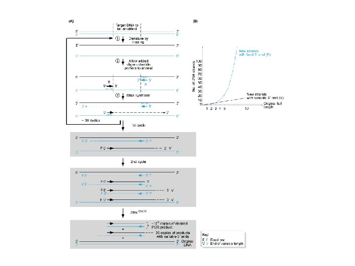
1° ciclo di PCR DNA genomico 5’ 3’ Primer reverse 3’ 5’ Primer forward DNA genomico 3’ 5’

ETEROGENEITA’ DEL TEMPLATO : ETEROZIGOSI PER UNA DELEZIONE C A G C A G C A C C T C A G G

F P M C/C G/- C/- LOSS OF HETEROZYGOSITY

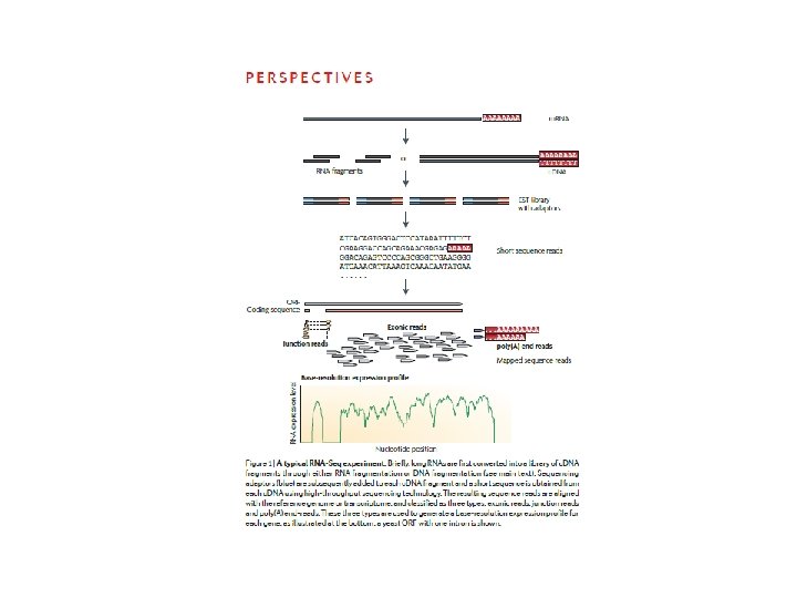
RNA sequencing Dopo trascrizione inversa

6 8 6 7 7/- 8 CTT 7/- -/-

Figure 1: Illumina Flow Cell Figure 2: Prepare Genomic DNA Sample DNA Figure 3: Attach DNA to Adapters Surface DNA Dense lawn of primers Figure 4: Bridge Amplification Adapters

Figure 5: Fragments Become Double Stranded Attached terminus Figure 6: Denature the Double-Standed Molecules Attached terminus Free terminus Attached Figure 7: Complete Amplification Figure 8: Determine First Base Clusters Laser

Figure 9: Image First Base Figure 10: Determine Second Base Figure 11: Image Second Chemistry Cycle Figure 12: Sequencing Over Multiple Chemistry Cycles Figure 13: Align Data Laser GCTGA. . .

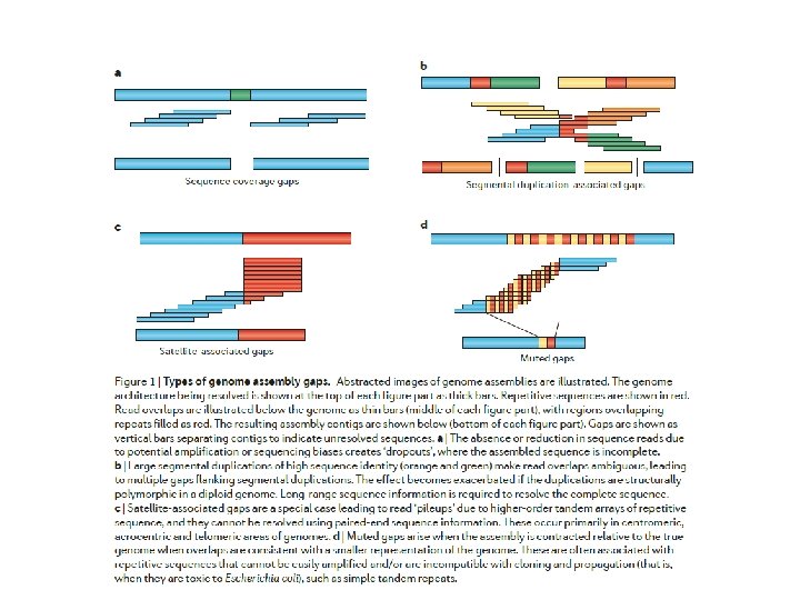
Figure 3 | Genome assembly algorithms. A genome schematic is shown at the top with four unique regions (blue, violet, green and yellow) and two copies of a repeated region (red). Three different strategies for genome assembly are outlined below this schematic. a | Overlap-layout-consensus (OLC). All pairwise alignments (arrows) between reads (solid bars) are detected. Reads are merged into contigs (below the vertical arrow) until a read at a repeat boundary (split colour bar) is detected, leading to a repeat that is unresolved and collapsed into a single copy. b | de Bruijn assembly. Reads are decomposed into overlapping k‑mers. An example of the decomposition for k = 3 nucleotides is shown, although in practice k ranges between 31 and 200 nucleotides. Identical k‑mers are merged and connected by an edge when appearing adjacently in reads. Contigs are formed by merging chains of k‑mers until repeat boundaries are reached. If a k‑mer appears in multiple positions (red segment) in the genome, it will fragment assemblies and additional graph operations must be applied to resolve such small repeats. The k‑mer approach is ideal for short-read data generated by massively parallel sequencing (MPS). c | String graph. Alignments that may be transitively inferred from all pairwise alignments are removed (grey arrows). A graph is created with a vertex for the endpoint of every read. Edges are created both for each unaligned interval of a read and for each remaining pairwise overlap. Vertices connect edges that correspond to the reads that overlap. When there is allelic variation, alternative paths in the graph are formed. Not shown, but common to all three algorithms, is the use of read pairs to produce the final assembly product.