Segmentation Market Segmentation All markets are heterogeneous and

Segmentation

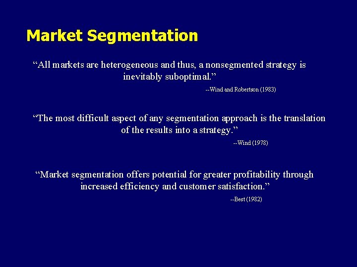
Market Segmentation “All markets are heterogeneous and thus, a nonsegmented strategy is inevitably suboptimal. ” --Wind and Robertson (1983) “The most difficult aspect of any segmentation approach is the translation of the results into a strategy. ” --Wind (1978) “Market segmentation offers potential for greater profitability through increased efficiency and customer satisfaction. ” --Best (1982)

Benefits of Market Segmentation 1. Helps in the design of marketing programs that are most effective for reaching homogeneous groups of customers. 2. Improves the strategic allocation of marketing resources. 3. Identifies opportunities for new product development. Methodologies: • Automatic Interaction Detector (AID) • Chi-Squared Automatic Interaction Detector (CHAID) • Regression and Discriminant Analysis • Hierarchical clustering (group similar items)

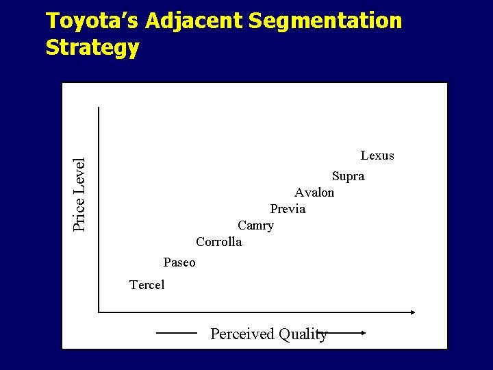
Toyota’s Adjacent Segmentation Strategy Price Level Lexus Supra Avalon Previa Camry Corrolla Paseo Tercel Perceived Quality

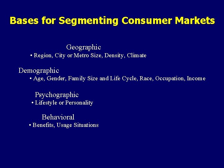
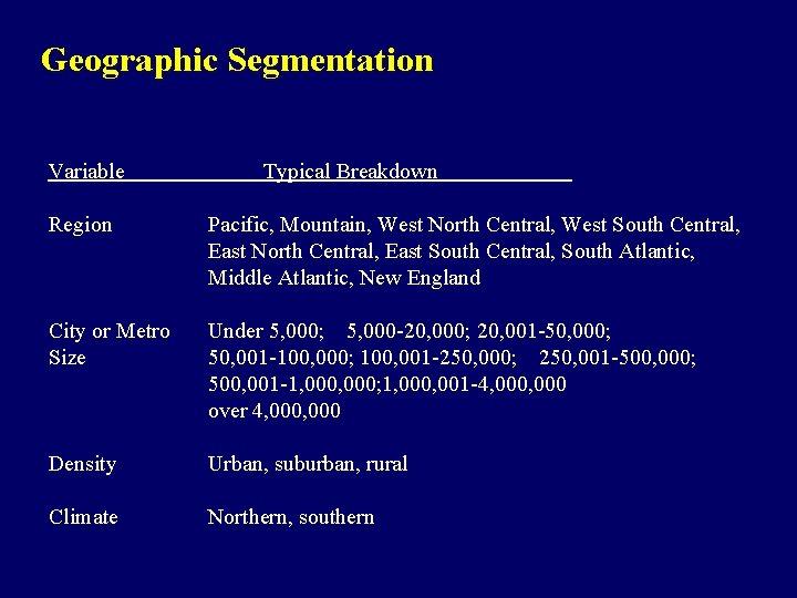
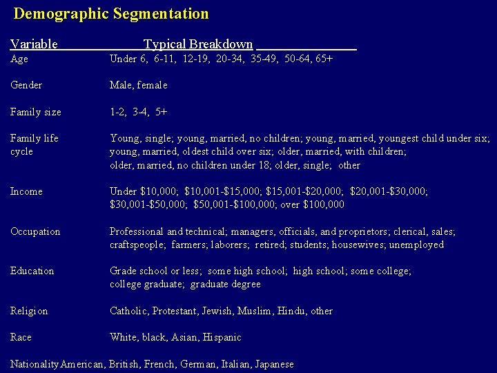
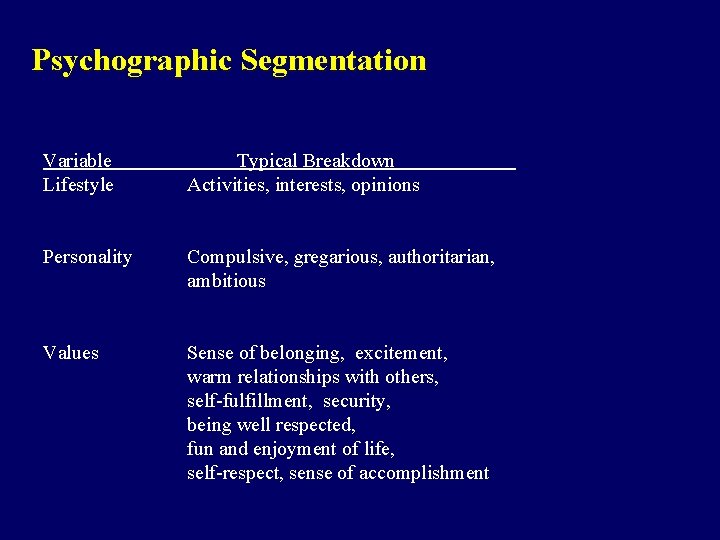
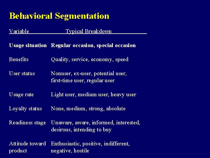
Bases for Segmenting Consumer Markets Geographic • Region, City or Metro Size, Density, Climate Demographic • Age, Gender, Family Size and Life Cycle, Race, Occupation, Income Psychographic • Lifestyle or Personality Behavioral • Benefits, Usage Situations

Geographic Segmentation Variable Typical Breakdown Region Pacific, Mountain, West North Central, West South Central, East North Central, East South Central, South Atlantic, Middle Atlantic, New England City or Metro Size Under 5, 000; 5, 000 -20, 000; 20, 001 -50, 000; 50, 001 -100, 000; 100, 001 -250, 000; 250, 001 -500, 000; 500, 001 -1, 000; 1, 000, 001 -4, 000 over 4, 000 Density Urban, suburban, rural Climate Northern, southern

Demographic Segmentation Variable Typical Breakdown Age Under 6, 6 -11, 12 -19, 20 -34, 35 -49, 50 -64, 65+ Gender Male, female Family size 1 -2, 3 -4, 5+ Family life cycle Young, single; young, married, no children; young, married, youngest child under six; young, married, oldest child over six; older, married, with children; older, married, no children under 18; older, single; other Income Under $10, 000; $10, 001 -$15, 000; $15, 001 -$20, 000; $20, 001 -$30, 000; $30, 001 -$50, 000; $50, 001 -$100, 000; over $100, 000 Occupation Professional and technical; managers, officials, and proprietors; clerical, sales; craftspeople; farmers; laborers; retired; students; housewives; unemployed Education Grade school or less; some high school; some college; college graduate; graduate degree Religion Catholic, Protestant, Jewish, Muslim, Hindu, other Race White, black, Asian, Hispanic Nationality. American, British, French, German, Italian, Japanese

Psychographic Segmentation Variable Lifestyle Typical Breakdown Activities, interests, opinions Personality Compulsive, gregarious, authoritarian, ambitious Values Sense of belonging, excitement, warm relationships with others, self-fulfillment, security, being well respected, fun and enjoyment of life, self-respect, sense of accomplishment

Behavioral Segmentation Variable Typical Breakdown Usage situation Regular occasion, special occasion Benefits Quality, service, economy, speed User status Nonuser, ex-user, potential user, first-time user, regular user Usage rate Light user, medium user, heavy user Loyalty status None, medium, strong, absolute Readiness stage Unaware, informed, interested, desirous, intending to buy Attitude toward Enthusiastic, positive, indifferent, product negative, hostile

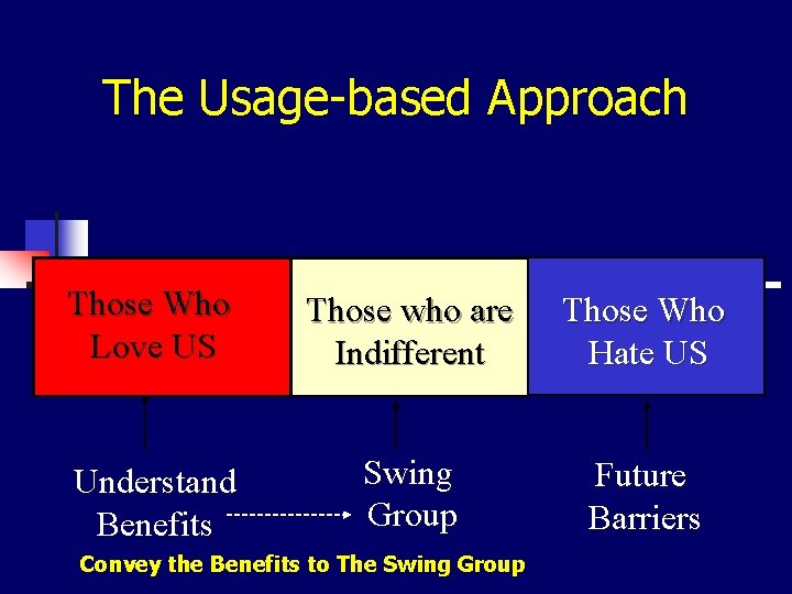
The Usage-based Approach Those Who Love US Those who are Indifferent Those Who Hate US Understand Benefits Swing Group Future Barriers Convey the Benefits to The Swing Group

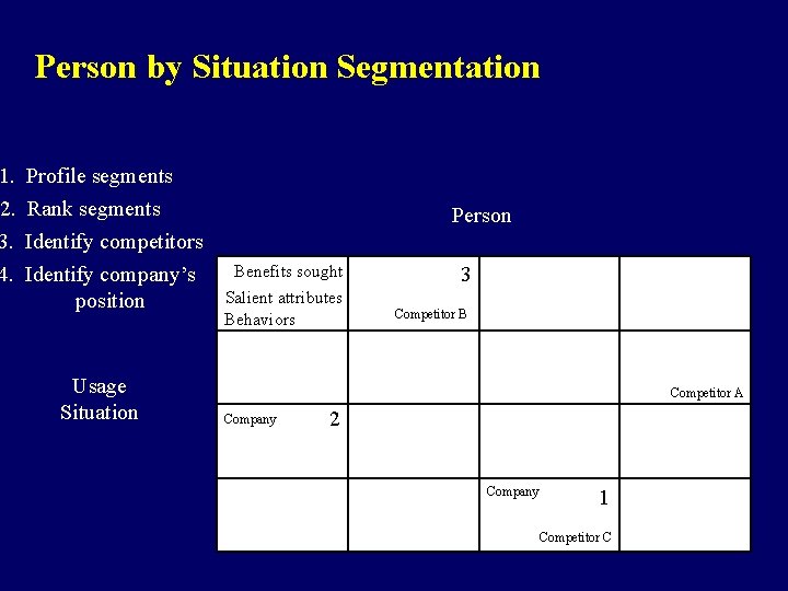
1. 2. 3. 4. Person by Situation Segmentation Profile segments Rank segments Identify competitors Identify company’s position Usage Situation Person Benefits sought Salient attributes Behaviors 3 Competitor B Competitor A Company 2 Company 1 Competitor C

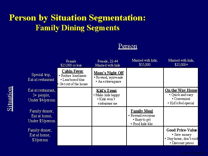
Person by Situation Segmentation: Family Dining Segments Person Female $25, 000 or less Situation Special trip, Eat at restaurant, 3+ people, Under $4/person Family dinner, Eat at home, Under $5/person Family dinner, Eat at home, $3/person Cabin Fever • Reduce loneliness • Less bored blue • Get out of the house Female, 22 -44 Married with kids, $35, 000 Married with kids, $25, 000+ Mom’s Night Off • Reward, rejuvenate • An extravagance On the Way Home Kid’s Treat • Quick and easy • Convenient • Kid’s feel special • Make kids happy • Kids won’t embarrass me Family Meal • Reward everyone • Easy to get • Food kids like Good Price-Value • Save money • Stay home, don’t cook • Discount prices Source: Pizza Hut

Market Segmentation n Cluster Analysis n n Hierarchical Clustering (exploratory) K-Means Clustering (confirmatory)

Cluster Analysis n n Cluster analysis is a class of techniques used to classify objects or cases into relatively homogeneous groups called clusters. Objects in each cluster tend to be similar to each other and dissimilar to objects in the other clusters. Cluster analysis is also called classification analysis, or numerical taxonomy. Both cluster analysis and discriminant analysis are concerned with classification. However, discriminant analysis requires prior knowledge of the cluster or group membership for each object or case included, to develop the classification rule. In contrast, in cluster analysis there is no a priori information about the group or cluster membership for any of the objects. Groups or clusters are suggested by the data, not defined a priori.

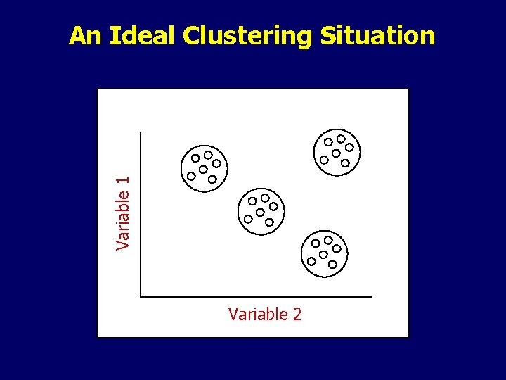
Variable 1 An Ideal Clustering Situation Variable 2

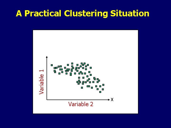
Variable 1 A Practical Clustering Situation Variable 2 X

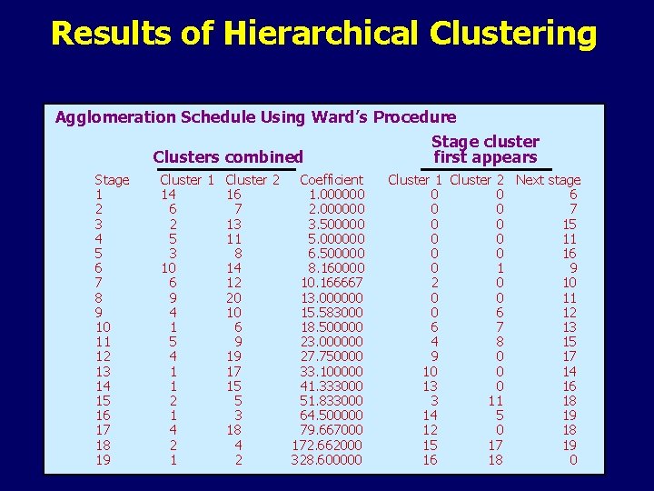
Statistics Associated with Cluster Analysis n n Agglomeration schedule. An agglomeration schedule gives information on the objects or cases being combined at each stage of a hierarchical clustering process. Cluster centroid. The cluster centroid is the mean values of the variables for all the cases or objects in a particular cluster. Cluster centers. The cluster centers are the initial starting points in nonhierarchical clustering. Clusters are built around these centers, or seeds. Cluster membership indicates the cluster to which each object or case belongs.

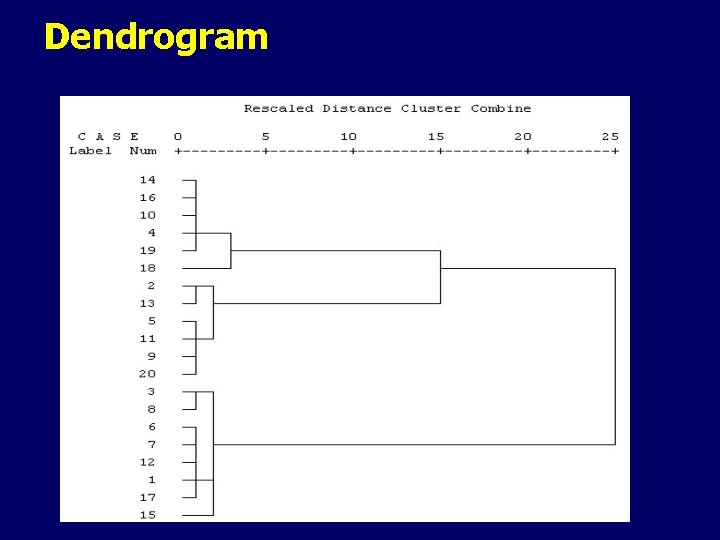
Statistics Associated with Cluster Analysis n n Dendrogram. A dendrogram, or tree graph, is a graphical device for displaying clustering results. Vertical lines represent clusters that are joined together. The position of the line on the scale indicates the distances at which clusters were joined. The dendrogram is read from left to right. Distances between cluster centers. These distances indicate how separated the individual pairs of clusters are. Clusters that are widely separated are distinct, and therefore desirable.

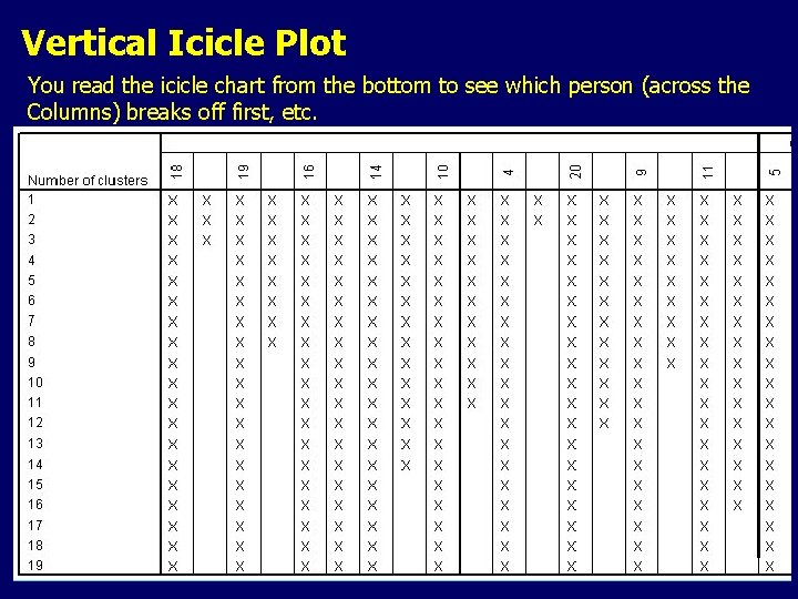
Statistics Associated with Cluster Analysis n n Icicle diagram. An icicle diagram is a graphical display of clustering results, so called because it resembles a row of icicles hanging from the eaves of a house. The columns correspond to the objects being clustered, and the rows correspond to the number of clusters. An icicle diagram is read from bottom to top. Figure 20. 7 is an icicle diagram. Similarity/distance coefficient matrix. A similarity/distance coefficient matrix is a lower-triangle matrix containing pairwise distances between objects or cases.

Conducting Cluster Analysis Formulate the Problem n n Perhaps the most important part of formulating the clustering problem is selecting the variables on which the clustering is based. Inclusion of even one or two irrelevant variables may distort an otherwise useful clustering solution. Basically, the set of variables selected should describe the similarity between objects in terms that are relevant to the marketing research problem. The variables should be selected based on past research, theory, or a consideration of the hypotheses being tested. In exploratory research, the researcher should exercise judgment and intuition.

Conducting Cluster Analysis Select a Distance or Similarity Measure n n n The most commonly used measure of similarity is the Euclidean distance or its square. The Euclidean distance is the square root of the sum of the squared differences in values for each variable. Other distance measures are also available. The city-block or Manhattan distance between two objects is the sum of the absolute differences in values for each variable. The Chebychev distance between two objects is the maximum absolute difference in values for any variable. If the variables are measured in vastly different units, the clustering solution will be influenced by the units of measurement. In these cases, before clustering respondents, we must standardize the data by rescaling each variable to have a mean of zero and a standard deviation of unity. It is also desirable to eliminate outliers (cases with atypical values). Use of different distance measures may lead to different clustering results. Hence, it is advisable to use different measures and compare the results.

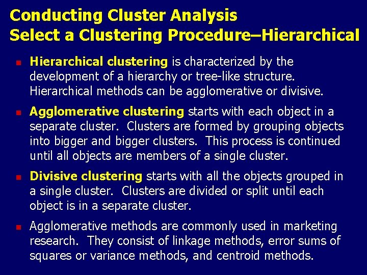
Conducting Cluster Analysis Select a Clustering Procedure–Hierarchical n n Hierarchical clustering is characterized by the development of a hierarchy or tree-like structure. Hierarchical methods can be agglomerative or divisive. Agglomerative clustering starts with each object in a separate cluster. Clusters are formed by grouping objects into bigger and bigger clusters. This process is continued until all objects are members of a single cluster. Divisive clustering starts with all the objects grouped in a single cluster. Clusters are divided or split until each object is in a separate cluster. Agglomerative methods are commonly used in marketing research. They consist of linkage methods, error sums of squares or variance methods, and centroid methods.

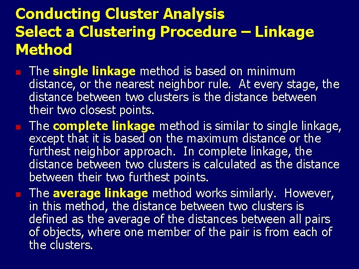
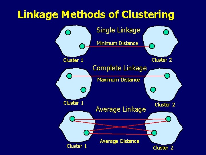
Conducting Cluster Analysis Select a Clustering Procedure – Linkage Method n n n The single linkage method is based on minimum distance, or the nearest neighbor rule. At every stage, the distance between two clusters is the distance between their two closest points. The complete linkage method is similar to single linkage, except that it is based on the maximum distance or the furthest neighbor approach. In complete linkage, the distance between two clusters is calculated as the distance between their two furthest points. The average linkage method works similarly. However, in this method, the distance between two clusters is defined as the average of the distances between all pairs of objects, where one member of the pair is from each of the clusters.

Linkage Methods of Clustering Single Linkage Minimum Distance Cluster 2 Cluster 1 Complete Linkage Maximum Distance Cluster 1 Average Linkage Cluster 2 Average Distance Cluster 2

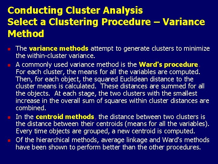
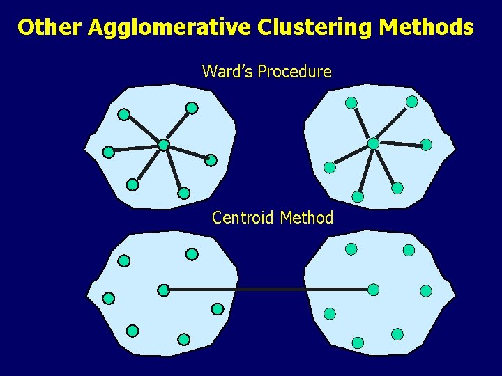
Conducting Cluster Analysis Select a Clustering Procedure – Variance Method n n The variance methods attempt to generate clusters to minimize the within-cluster variance. A commonly used variance method is the Ward's procedure. For each cluster, the means for all the variables are computed. Then, for each object, the squared Euclidean distance to the cluster means is calculated. These distances are summed for all the objects. At each stage, the two clusters with the smallest increase in the overall sum of squares within cluster distances are combined. In the centroid methods, the distance between two clusters is the distance between their centroids (means for all the variables). Every time objects are grouped, a new centroid is computed. Of the hierarchical methods, average linkage and Ward's methods have been shown to perform better than the other procedures.

Other Agglomerative Clustering Methods Ward’s Procedure Centroid Method

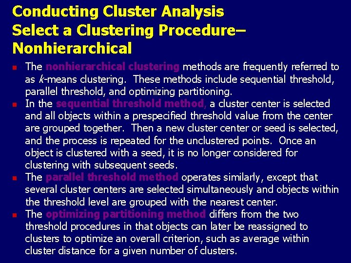
Conducting Cluster Analysis Select a Clustering Procedure– Nonhierarchical n n The nonhierarchical clustering methods are frequently referred to as k-means clustering. These methods include sequential threshold, parallel threshold, and optimizing partitioning. In the sequential threshold method, a cluster center is selected and all objects within a prespecified threshold value from the center are grouped together. Then a new cluster center or seed is selected, and the process is repeated for the unclustered points. Once an object is clustered with a seed, it is no longer considered for clustering with subsequent seeds. The parallel threshold method operates similarly, except that several cluster centers are selected simultaneously and objects within the threshold level are grouped with the nearest center. The optimizing partitioning method differs from the two threshold procedures in that objects can later be reassigned to clusters to optimize an overall criterion, such as average within cluster distance for a given number of clusters.

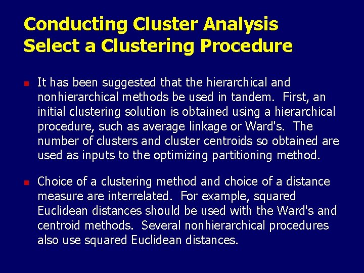
Conducting Cluster Analysis Select a Clustering Procedure n n It has been suggested that the hierarchical and nonhierarchical methods be used in tandem. First, an initial clustering solution is obtained using a hierarchical procedure, such as average linkage or Ward's. The number of clusters and cluster centroids so obtained are used as inputs to the optimizing partitioning method. Choice of a clustering method and choice of a distance measure are interrelated. For example, squared Euclidean distances should be used with the Ward's and centroid methods. Several nonhierarchical procedures also use squared Euclidean distances.

Results of Hierarchical Clustering Agglomeration Schedule Using Ward’s Procedure Stage cluster Clusters combined first appears Stage 1 2 3 4 5 6 7 8 9 10 11 12 13 14 15 16 17 18 19 Cluster 1 Cluster 2 Coefficient 14 16 1. 000000 6 7 2. 000000 2 13 3. 500000 5 11 5. 000000 3 8 6. 500000 10 14 8. 160000 6 12 10. 166667 9 20 13. 000000 4 10 15. 583000 1 6 18. 500000 5 9 23. 000000 4 19 27. 750000 1 17 33. 100000 1 15 41. 333000 2 5 51. 833000 1 3 64. 500000 4 18 79. 667000 2 4 172. 662000 1 2 328. 600000 Cluster 1 Cluster 2 Next stage 0 0 6 0 0 7 0 0 15 0 0 11 0 0 16 0 1 9 2 0 10 0 0 11 0 6 12 6 7 13 4 8 15 9 0 17 10 0 14 13 0 16 3 11 18 14 5 19 12 0 18 15 17 19 16 18 0

Vertical Icicle Plot You read the icicle chart from the bottom to see which person (across the Columns) breaks off first, etc.

Dendrogram

Conducting Cluster Analysis Decide on the Number of Clusters n n Theoretical, conceptual, or practical considerations may suggest a certain number of clusters. In hierarchical clustering, the distances at which clusters are combined can be used as criteria. This information can be obtained from the agglomeration schedule or from the dendrogram. In nonhierarchical clustering, the ratio of total withingroup variance to between-group variance can be plotted against the number of clusters. The point at which an elbow or a sharp bend occurs indicates an appropriate number of clusters. The relative sizes of the clusters should be meaningful.

Conducting Cluster Analysis Interpreting and Profiling the Clusters n n Interpreting and profiling clusters involves examining the cluster centroids. The centroids enable us to describe each cluster by assigning it a name or label. It is often helpful to profile the clusters in terms of variables that were not used for clustering. These may include demographic, psychographic, product usage, media usage, or other variables. n We often use Compare Means to do the profiling

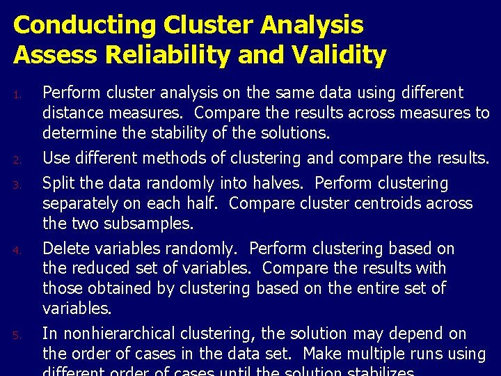
Conducting Cluster Analysis Assess Reliability and Validity 1. 2. 3. 4. 5. Perform cluster analysis on the same data using different distance measures. Compare the results across measures to determine the stability of the solutions. Use different methods of clustering and compare the results. Split the data randomly into halves. Perform clustering separately on each half. Compare cluster centroids across the two subsamples. Delete variables randomly. Perform clustering based on the reduced set of variables. Compare the results with those obtained by clustering based on the entire set of variables. In nonhierarchical clustering, the solution may depend on the order of cases in the data set. Make multiple runs using

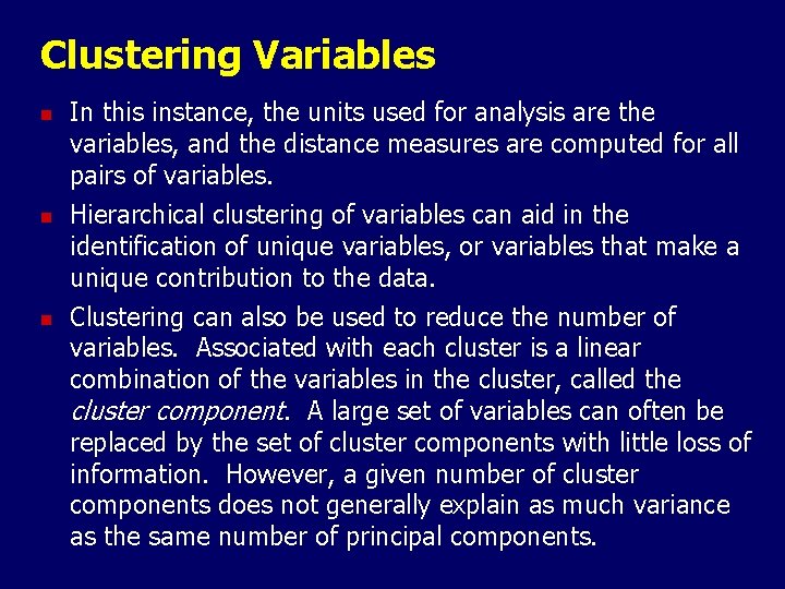
Clustering Variables n n n In this instance, the units used for analysis are the variables, and the distance measures are computed for all pairs of variables. Hierarchical clustering of variables can aid in the identification of unique variables, or variables that make a unique contribution to the data. Clustering can also be used to reduce the number of variables. Associated with each cluster is a linear combination of the variables in the cluster, called the cluster component. A large set of variables can often be replaced by the set of cluster components with little loss of information. However, a given number of cluster components does not generally explain as much variance as the same number of principal components.

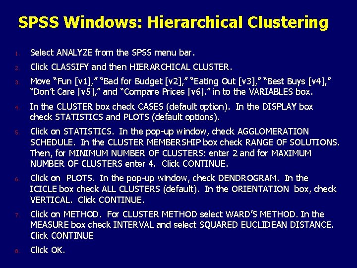
SPSS Windows: Hierarchical Clustering 1. Select ANALYZE from the SPSS menu bar. 2. Click CLASSIFY and then HIERARCHICAL CLUSTER. 3. 4. 5. 6. 7. 8. Move “Fun [v 1], ” “Bad for Budget [v 2], ” “Eating Out [v 3], ” “Best Buys [v 4], ” “Don’t Care [v 5], ” and “Compare Prices [v 6]. ” in to the VARIABLES box. In the CLUSTER box check CASES (default option). In the DISPLAY box check STATISTICS and PLOTS (default options). Click on STATISTICS. In the pop-up window, check AGGLOMERATION SCHEDULE. In the CLUSTER MEMBERSHIP box check RANGE OF SOLUTIONS. Then, for MINIMUM NUMBER OF CLUSTERS: enter 2 and for MAXIMUM NUMBER OF CLUSTERS enter 4. Click CONTINUE. Click on PLOTS. In the pop-up window, check DENDROGRAM. In the ICICLE box check ALL CLUSTERS (default). In the ORIENTATION box, check VERTICAL. Click CONTINUE. Click on METHOD. For CLUSTER METHOD select WARD’S METHOD. In the MEASURE box check INTERVAL and select SQUARED EUCLIDEAN DISTANCE. Click CONTINUE Click OK.

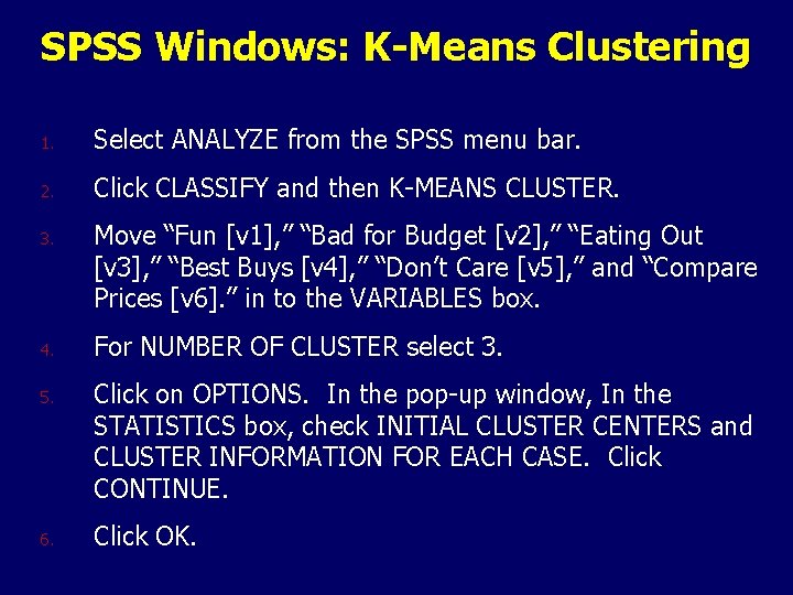
SPSS Windows: K-Means Clustering 1. Select ANALYZE from the SPSS menu bar. 2. Click CLASSIFY and then K-MEANS CLUSTER. 3. 4. 5. 6. Move “Fun [v 1], ” “Bad for Budget [v 2], ” “Eating Out [v 3], ” “Best Buys [v 4], ” “Don’t Care [v 5], ” and “Compare Prices [v 6]. ” in to the VARIABLES box. For NUMBER OF CLUSTER select 3. Click on OPTIONS. In the pop-up window, In the STATISTICS box, check INITIAL CLUSTER CENTERS and CLUSTER INFORMATION FOR EACH CASE. Click CONTINUE. Click OK.