Searching for Solutions Artificial Intelligence CSPP 56553 January

Searching for Solutions Artificial Intelligence CSPP 56553 January 14, 2004

Agenda • Search – Motivation – Problem-solving agents – Rigorous problem definitions • Exhaustive search: – Breadth-first, Depth-first, Iterative Deepening – Search analysis: Computational cost, limitations • Efficient, Optimal Search – Hill-climbing, A* • Game play: Search for the best move – Minimax, Alpha-Beta, Expectiminimax

Problem-Solving Agents • Goal-based agents – Identify goal, sequence of actions that satisfy • Goal: set of satisfying world states – Precise specification of what to achieve • Problem formulation: – Identify states and actions to consider in achieving goal – Given a set of actions, consider sequence of actions leading to a state with some value • Search: Process of looking for sequence – Problem -> action sequence solution

Agent Environment Specification ● Dimensions – Fully observable vs partially observable: – – Deterministic vs stochastic: – – Static Discrete vs continuous: – ● Deterministic Static vs dynamic: – – Fully Discrete Issues?

Closer to Reality • Sensorless agents (conformant problems) – Replace state with “belief state” • Multiple physical states, successors: sets of successors • Partial observability (contigency problems) – Solution is tree, branch chosen based on percepts

Formal Problem Definitions • Key components: – Initial state: • E. g. First location – Available actions: • Successor function: reachable states – Goal test: • Conditions for goal satisfaction – Path cost: • Cost of sequence from initial state to reachable state • Solution: Path from initial state to goal – Optimal if lowest cost

Why Search? • Not just city route search – Many AI problems can be posed as search • What are some examples? • How can we formulate the problem?

Basic Search Algorithm • Form a 1 -element queue of 0 cost=root node • Until first path in queue ends at goal or no paths – Remove 1 st path from queue; extend path one step Paths to extend – Reject all paths with loops Order of paths added – Add new paths to queue Position new paths added • If goal found=>success; else, failure

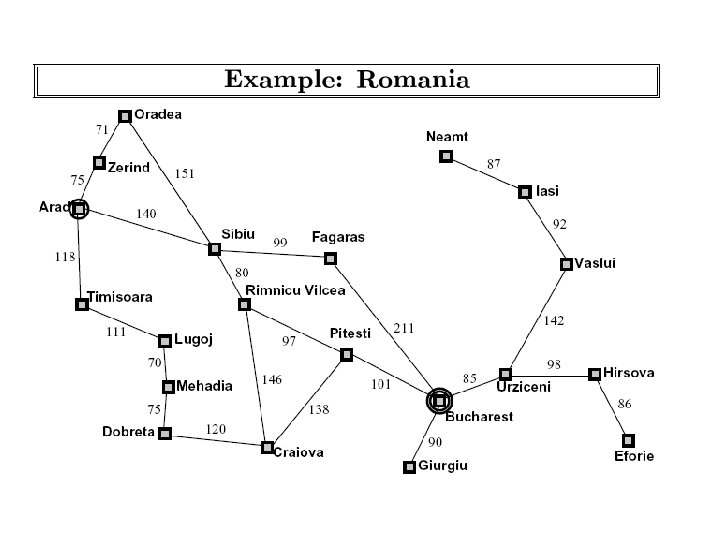
Basic Search Problem • Vertices: Cities; Edges: Steps to next, distance • Find route from S(tart) to G(oal) 4 4 3 5 4 2 4 3

Formal Statement • Initial State: in(S) • Successor function: – Go to all neighboring nodes • Goal state: in(G) • Path cost: – Sum of edge costs

Breadth-first Search • Explore all paths to a given depth

Breadth-first Search Algorithm • Form a 1 -element queue of 0 cost=root node • Until first path in queue ends at goal or no paths – Remove 1 st path from queue; extend path one step – Reject all paths with loops – Add new paths to BACK of queue • If goal found=>success; else, failure

Analyzing Search Algorithms • Criteria: – Completeness: Finds a solution if one exists – Optimal: Find the best (least cost) solution – Time complexity: Order of growth of running time – Space complexity: Order of growth of space needs • BFS: – Complete: yes; Optimal: only if # steps= cost – Time complexity: O(b^d+1); Space: O(b^d+1)

Depth-first Search • Pick a child of each node visited, go forward – Ignore alternatives until exhaust path w/o goal

Depth-first Search Algorithm • Form a 1 -element queue of 0 cost=root node • Until first path in queue ends at goal or no paths – Remove 1 st path from queue; extend path one step – Reject all paths with loops – Add new paths to FRONT of queue • If goal found=>success; else, failure

Question • Why might you choose DFS vs BFS? – Vice versa?

Search Issues • Breadth-first search: – Good if many (effectively) infinite paths, b<< – Bad if many end at same short depth, b>> • Depth-first search: – Good if: most partial=>complete, not too long – Bad if many (effectively) infinite paths

Iterative Deepening • Problem: – DFS good space behavior • Could go down blind path, or sub-optimal • Solution: – Search at progressively greater depths: • 1, 2, 3, 4, 5…. .

Question • Is this wasting a lot of work?

Progressive Deepening • Answer: (surprisingly) No! – Assume cost of actions at leaves dominates – Last ply (depth d): Cost = b^d – Preceding plies: b^0 + b^1+…b^(d-1) • (b^d - 1)/(b -1) – Ratio of last ply cost/all preceding ~ b - 1 – For large branching factors, prior work small relative to final ply

Informed and Optimal Search • Roadmap – Heuristics: Admissible, Consistent – Hill-Climbing – A* – Analysis

Heuristic Search • A little knowledge is a powerful thing – Order choices to explore better options first – More knowledge => less search – Better search alg? ? Better search space • Measure of remaining cost to goal-heuristic – E. g. actual distance => straight-line distance A S B 10. 4 6. 7 C 4. 0 11. 0 G 3. 0 8. 9 D E 6. 9 F

Hill-climbing Search • Select child to expand that is closest to goal S 10. 4 A D 10. 4 A 6. 7 B 8. 9 E 3. 0 6. 9 F G

Hill-climbing Search Algorithm • Form a 1 -element queue of 0 cost=root node • Until first path in queue ends at goal or no paths – Remove 1 st path from queue; extend path one step – Reject all paths with loops – Sort new paths by estimated distance to goal – Add new paths to FRONT of queue • If goal found=>success; else, failure

Heuristic Search Issues • Parameter-oriented hill climbing – Make one step adjustments to all parameters • E. g. tuning brightness, contrast, r, g, b on TV – Test effect on performance measure • Problems: – Foothill problem: aka local maximum • All one-step changes - worse!, but not global max – Plateau problem: one-step changes, no FOM + – Ridge problem: all one-steps down, but not even local max • Solution (local max): Randomize!!

Search Costs

Optimal Search • Find BEST path to goal – Find best path EFFICIENTLY • Exhaustive search: – Try all paths: return best • Optimal paths with less work: – Expand shortest paths – Expand shortest expected paths – Eliminate repeated work - dynamic programming

Efficient Optimal Search • Find best path without exploring all paths – Use knowledge about path lengths • Maintain path & path length – Expand shortest paths first – Halt if partial path length > complete path length

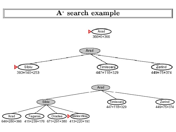
Underestimates • Improve estimate of complete path length – Add (under)estimate of remaining distance – u(total path dist) = d(partial path)+u(remaining) – Underestimates must ultimately yield shortest – Stop if all u(total path dist) > d(complete path) • Straight-line distance => underestimate • Better estimate => Better search • No missteps

Search with Dynamic Programming • Avoid duplicating work – Dynamic Programming principle: • Shortest path from S to G through I is shortest path from S to I plus shortest path from I to G • No need to consider other routes to or from I

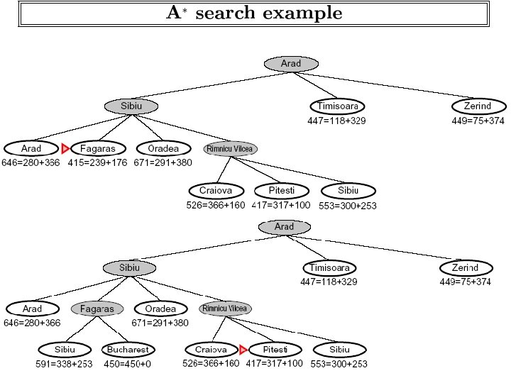
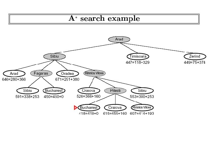
A* Search Algorithm • Combines good optimal search ideas – Dynamic programming and underestimates • Form a 1 -element queue of 0 cost=root node • Until first path in queue ends at goal or no paths – Remove 1 st path from queue; extend path one step – Reject all paths with loops • For all paths with same terminal node, keep only shortest – Add new paths to queue – Sort all paths by total length underestimate, shortest first (d(partial path) + u(remaining)) • If goal found=>success; else, failure

Heuristics • A* search: only as good as the heuristic • Heuristic requirements: – Admissible: • UNDERESTIMATE true remaining cost to goal – Consistent: • h(n) <= c(n, a, n') + h(n')

Constructing Heuristics • Relaxation: – State problem – Remove one or more constraints • What is the cost then? • Example: – 8 -square: Move A to B if • 1) A &B horizontally or vertically adjacent, and • 2) B is empty – Ignore 1) -> Manhattan distance – Ignore 1) & 2): # of misplaced squares

Game Play: Search for the Best Move

Agenda • Game search characteristics • Minimax procedure – Adversarial Search • Alpha-beta pruning: – “If it’s bad, we don’t need to know HOW awful!” • Game search specialties – Progressive deepening – Singular extensions

Games as Search • Nodes = Board Positions • Each ply (depth + 1) = Move • Special feature: – Two players, adversial • Static evaluation function – Instantaneous assessment of board configuration – NOT perfect (maybe not even very good)

Minimax Lookahead • Modeling adversarial players: – Maximizer = positive values – Minimizer = negative values • Decisions depend on choices of other player • Look forward to some limit – Static evaluate at limit – Propagate up via minimax

Minimax Procedure • If at limit of search, compute static value • Relative to player • If minimizing level, do minimax – Report minimum • If maximizing level, do minimax – Report maximum

Minimax Search

Minimax Analysis • Complete: – Yes, if finite tree • Optimal: – Yes, if optimal opponent • Time: – b^m • Space: – bm (progressive deepening DFS) • Practically: Chess: b~35, m~100 – Complete solution is impossible

Alpha-Beta Pruning • Alpha-beta principle: If you know it’s bad, don’t waste time finding out HOW bad • May eliminate some static evaluations • May eliminate some node expansions

Alpha-Beta Pruning

Alpha-Beta Pruning

Alpha-Beta Pruning

Alpha-Beta Pruning

Alpha-Beta Pruning

Alpha-Beta Procedure If level=TOP_LEVEL, alpha = NEGMAX; beta= POSMAX If (reached Search-limit), compute & return static value of current If level is minimizing level, While more children to explore AND alpha < beta ab = alpha-beta(child) if (ab < beta), then beta = ab Report beta If level is maximizing level, While more children to explore AND alpha < beta ab = alpha-beta(child) if (ab > alpha), then alpha = ab Report alpha

Alpha-Beta Pruning Analysis • Worst case: – Bad ordering: Alpha-beta prunes NO nodes • Best case: – Assume cooperative oracle orders nodes • Best value on left • “If an opponent has some response that makes move bad no matter what the moving player does, then the move is bad. ” • Implies: check move where opposing player has choice, check all own moves

Optimal Alpha-Beta Ordering 1 2 5 6 3 7 8 4 9 10 11 12 13 141516 171819 202122 232425 262728 293031 323334 353637 383940 14 15 16 17 18 19 20 21 22 13 14 15 26 27 28 29 30 31 13 14 15 35 36 37 38 39 40

Optimal Ordering Alpha-Beta • Significant reduction of work: – 11 of 27 static evaluations • Lower bound on # of static evaluations: – if d is even, s = 2*b^d/2 -1 – if d is odd, s = b^(d+1)/2+b^(d-1)/2 -1 • Upper bound on # of static evaluations: – b^d • Reality: somewhere between the two – Typically closer to best than worst

Heuristic Game Search • Handling time pressure – Focus search – Be reasonably sure “best” option found is likely to be a good option. • Progressive deepening – Always having a good move ready • Singular extensions – Follow out stand-out moves

Singular Extensions • Problem: Explore to some depth, but things change a lot in next ply – False sense of security – aka “horizon effect” • Solution: “Singular extensions” – If static value stands out, follow it out – Typically, “forced” moves: • E. g. follow out captures

Additional Pruning Heuristics • Tapered search: – Keep more branches for higher ranked children • Rank nodes cheaply • Rule out moves that look bad • Problem: – Heuristic: May be misleading • Could miss good moves

Deterministic Games

Games with Chance • Many games mix chance and strategy – E. g. Backgammon – Combine dice rolls + opponent moves • Modeling chance in game tree – For each ply, add another ply of “chance nodes” – Represent alternative rolls of dice • One branch per roll • Associate probability of roll with branch

Expectiminimax: Minimax+Chance • Adding chance to minimax – For each roll, compute max/min as before • Computing values at chance nodes – Calculate EXPECTED value – Sum of branches • Weight by probability of branch

Expecti… Tree

Summary • Game search: – Key features: Alternating, adversarial moves • Minimax search: Models adversarial game • Alpha-beta pruning: – If a branch is bad, don’t need to see how bad! – Exclude branch once know can’t change value – Can significantly reduce number of evaluations • Heuristics: Search under pressure – Progressive deepening; Singular extensions