Relational Normalization Theory Chapter 8 1 Limitations of

Relational Normalization Theory Chapter 8 1

Limitations of E-R Designs • Provides a set of guidelines, does not result in a unique database schema • Does not provide a way of evaluating alternative schemas • Normalization theory provides a mechanism for analyzing and refining the schema produced by an E-R design 2

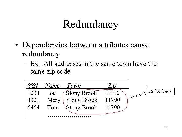
Redundancy • Dependencies between attributes cause redundancy – Ex. All addresses in the same town have the same zip code SSN Name Town 1234 Joe Stony Brook 4321 Mary Stony Brook 5454 Tom Stony Brook …………………. Zip 11790 Redundancy 3

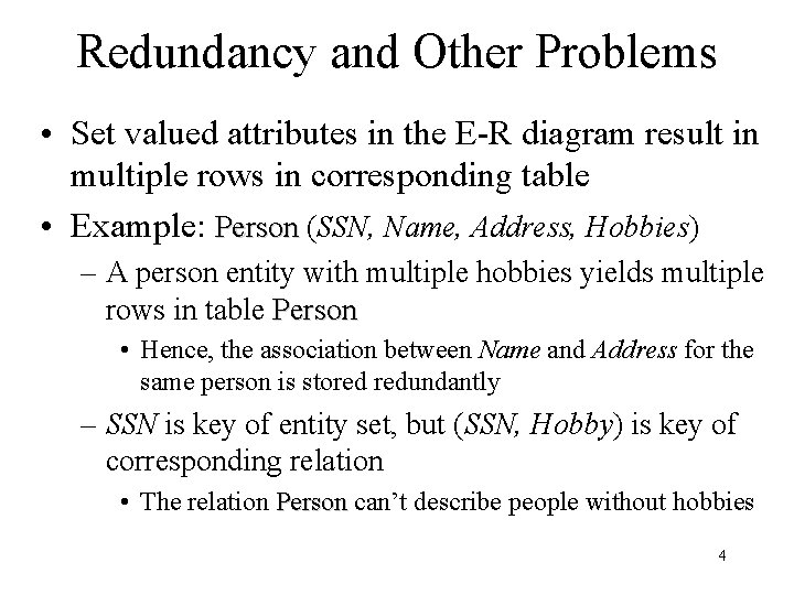
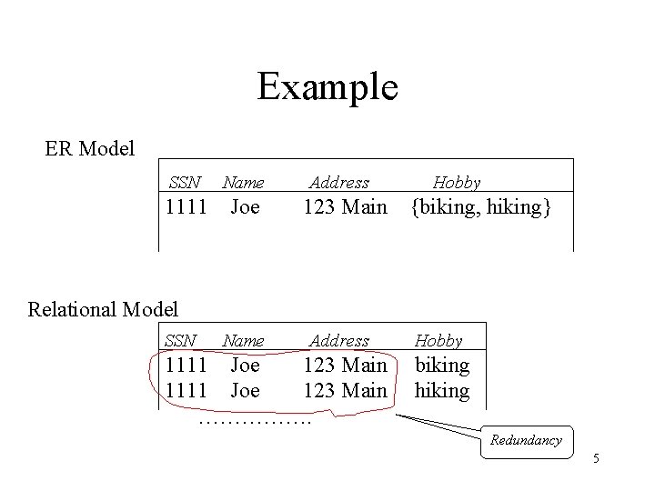
Redundancy and Other Problems • Set valued attributes in the E-R diagram result in multiple rows in corresponding table • Example: Person (SSN, Name, Address, Hobbies) – A person entity with multiple hobbies yields multiple rows in table Person • Hence, the association between Name and Address for the same person is stored redundantly – SSN is key of entity set, but (SSN, Hobby) is key of corresponding relation • The relation Person can’t describe people without hobbies 4

Example ER Model SSN Name 1111 Joe Address 123 Main Hobby {biking, hiking} Relational Model SSN Name Address 1111 Joe 123 Main ……………. Hobby biking hiking Redundancy 5

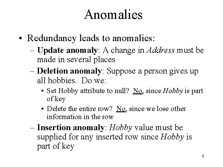
Anomalies • Redundancy leads to anomalies: – Update anomaly: A change in Address must be made in several places – Deletion anomaly: Suppose a person gives up all hobbies. Do we: • Set Hobby attribute to null? No, since Hobby is part of key • Delete the entire row? No, since we lose other information in the row – Insertion anomaly: Hobby value must be supplied for any inserted row since Hobby is part of key 6

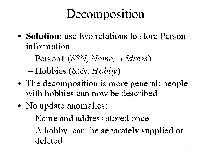
Decomposition • Solution: use two relations to store Person information – Person 1 (SSN, Name, Address) – Hobbies (SSN, Hobby) • The decomposition is more general: people with hobbies can now be described • No update anomalies: – Name and address stored once – A hobby can be separately supplied or deleted 7

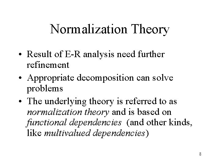
Normalization Theory • Result of E-R analysis need further refinement • Appropriate decomposition can solve problems • The underlying theory is referred to as normalization theory and is based on functional dependencies (and other kinds, like multivalued dependencies) dependencies 8

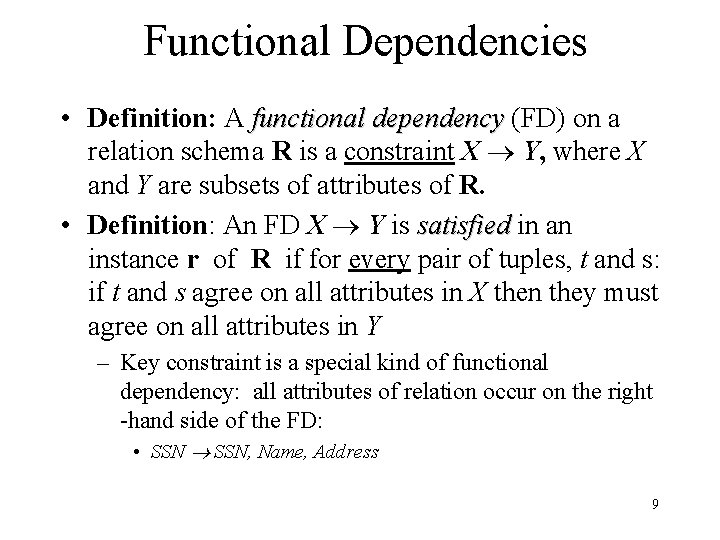
Functional Dependencies • Definition: A functional dependency (FD) on a relation schema R is a constraint X Y, where X and Y are subsets of attributes of R. • Definition: An FD X Y is satisfied in an instance r of R if for every pair of tuples, t and s: if t and s agree on all attributes in X then they must agree on all attributes in Y – Key constraint is a special kind of functional dependency: all attributes of relation occur on the right -hand side of the FD: • SSN, Name, Address 9

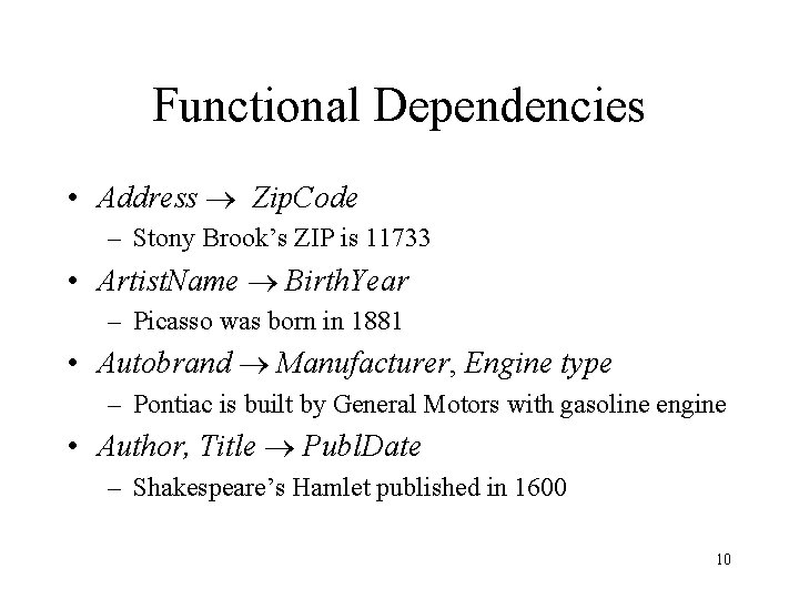
Functional Dependencies • Address Zip. Code – Stony Brook’s ZIP is 11733 • Artist. Name Birth. Year – Picasso was born in 1881 • Autobrand Manufacturer, Engine type – Pontiac is built by General Motors with gasoline engine • Author, Title Publ. Date – Shakespeare’s Hamlet published in 1600 10

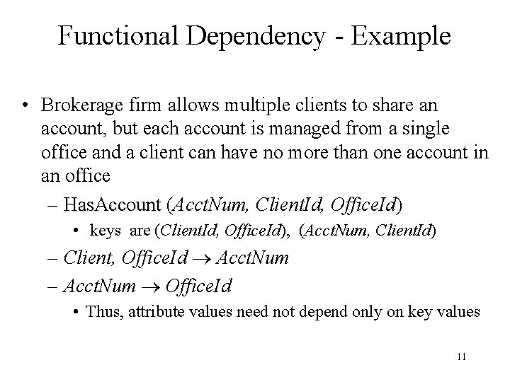
Functional Dependency - Example • Brokerage firm allows multiple clients to share an account, but each account is managed from a single office and a client can have no more than one account in an office – Has. Account (Acct. Num, Client. Id, Office. Id) • keys are (Client. Id, Office. Id), (Acct. Num, Client. Id) – Client, Office. Id Acct. Num – Acct. Num Office. Id • Thus, attribute values need not depend only on key values 11

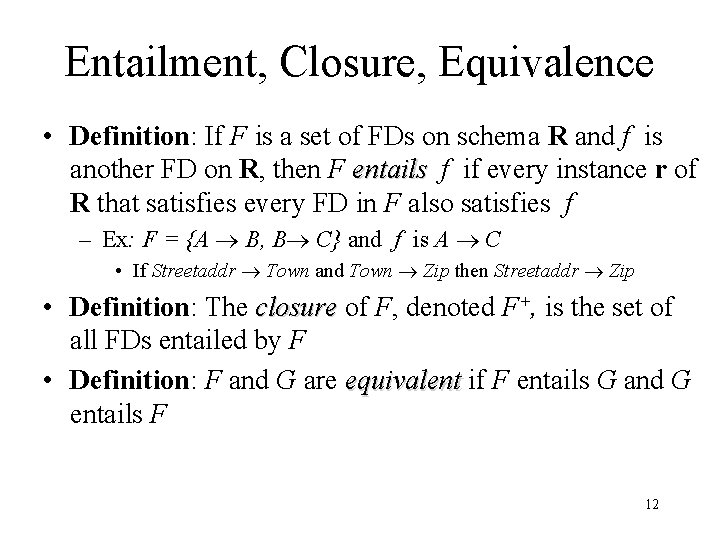
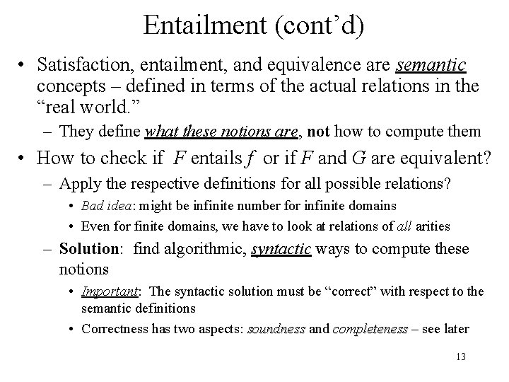
Entailment, Closure, Equivalence • Definition: If F is a set of FDs on schema R and f is another FD on R, then F entails f if every instance r of R that satisfies every FD in F also satisfies f – Ex: F = {A B, B C} and f is A C • If Streetaddr Town and Town Zip then Streetaddr Zip • Definition: The closure of F, denoted F+, is the set of all FDs entailed by F • Definition: F and G are equivalent if F entails G and G entails F 12

Entailment (cont’d) • Satisfaction, entailment, and equivalence are semantic concepts – defined in terms of the actual relations in the “real world. ” – They define what these notions are, not how to compute them • How to check if F entails f or if F and G are equivalent? – Apply the respective definitions for all possible relations? • Bad idea: might be infinite number for infinite domains • Even for finite domains, we have to look at relations of all arities – Solution: find algorithmic, syntactic ways to compute these notions • Important: The syntactic solution must be “correct” with respect to the semantic definitions • Correctness has two aspects: soundness and completeness – see later 13

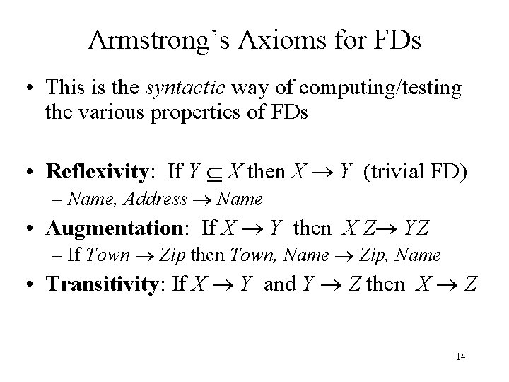
Armstrong’s Axioms for FDs • This is the syntactic way of computing/testing the various properties of FDs • Reflexivity: If Y X then X Y (trivial FD) – Name, Address Name • Augmentation: If X Y then X Z YZ – If Town Zip then Town, Name Zip, Name • Transitivity: If X Y and Y Z then X Z 14

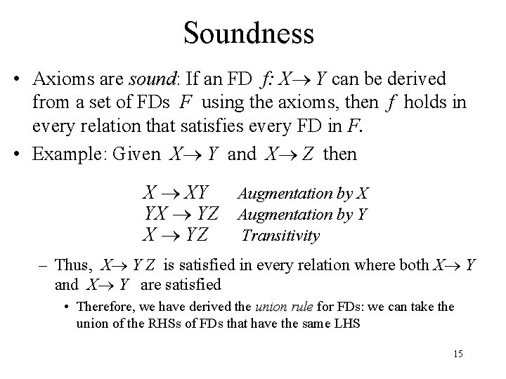
Soundness • Axioms are sound: sound If an FD f: X Y can be derived from a set of FDs F using the axioms, then f holds in every relation that satisfies every FD in F. • Example: Given X Y and X Z then X XY Augmentation by X YX YZ Augmentation by Y X YZ Transitivity – Thus, X Y Z is satisfied in every relation where both X Y and X Y are satisfied • Therefore, we have derived the union rule for FDs: we can take the union of the RHSs of FDs that have the same LHS 15

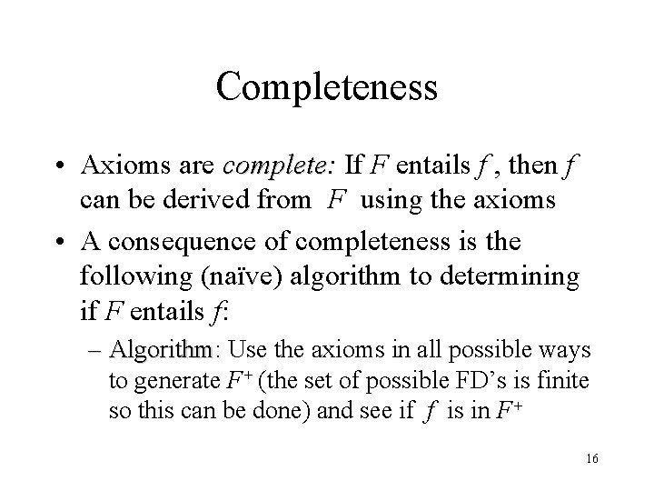
Completeness • Axioms are complete: complete If F entails f , then f can be derived from F using the axioms • A consequence of completeness is the following (naïve) algorithm to determining if F entails f: – Algorithm: Algorithm Use the axioms in all possible ways to generate F+ (the set of possible FD’s is finite so this can be done) and see if f is in F+ 16

Correctness • The notions of soundness and completeness link the syntax (Armstrong’s axioms) with semantics (the definitions in terms of relational instances) • This is a precise way of saying that the algorithm for entailment based on the axioms is “correct” with respect to the definitions 17

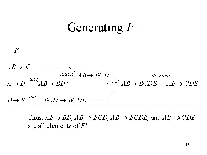
Generating + F F AB C A D D E aug union AB BCD AB BD trans decomp AB BCDE AB CDE BCDE Thus, AB BD, AB BCDE, and AB CDE are all elements of F+ 18

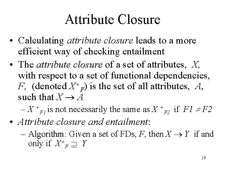
Attribute Closure • Calculating attribute closure leads to a more efficient way of checking entailment • The attribute closure of a set of attributes, X, with respect to a set of functional dependencies, F, (denoted X+F) is the set of all attributes, A, such that X A – X +F 1 is not necessarily the same as X +F 2 if F 1 F 2 • Attribute closure and entailment: – Algorithm: Algorithm Given a set of FDs, F, then X Y if and only if X+F Y 19

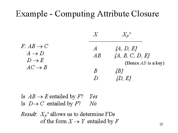
Example - Computing Attribute Closure X F: AB C A D D E AC B Is AB E entailed by F? Is D C entailed by F? A AB X F+ {A, D, E} {A, B, C, D, E} (Hence AB is a key) B D {B} {D, E} Yes No Result: XF+ allows us to determine FDs of the form X Y entailed by F 20

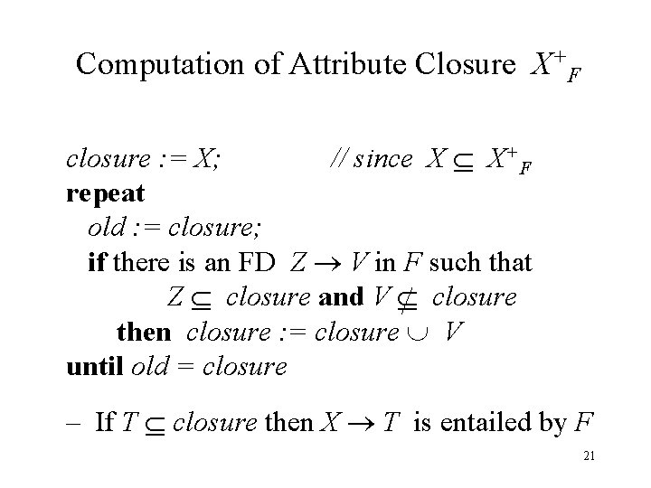
Computation of Attribute Closure X+F closure : = X; // since X X+F repeat old : = closure; if there is an FD Z V in F such that Z closure and V closure then closure : = closure V until old = closure – If T closure then X T is entailed by F 21

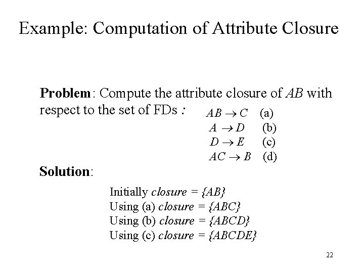
Example: Computation of Attribute Closure Problem: Compute the attribute closure of AB with respect to the set of FDs : AB C (a) A D (b) D E (c) AC B (d) Solution: Initially closure = {AB} Using (a) closure = {ABC} Using (b) closure = {ABCD} Using (c) closure = {ABCDE} 22

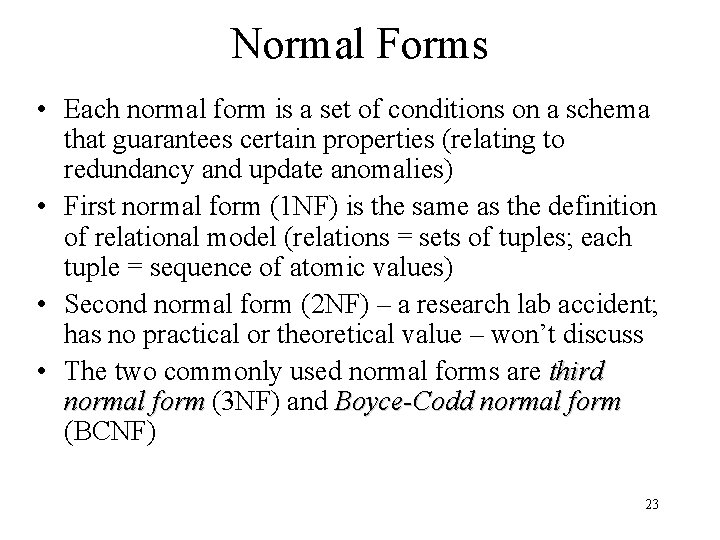
Normal Forms • Each normal form is a set of conditions on a schema that guarantees certain properties (relating to redundancy and update anomalies) • First normal form (1 NF) is the same as the definition of relational model (relations = sets of tuples; each tuple = sequence of atomic values) • Second normal form (2 NF) – a research lab accident; has no practical or theoretical value – won’t discuss • The two commonly used normal forms are third normal form (3 NF) and Boyce-Codd normal form (BCNF) 23

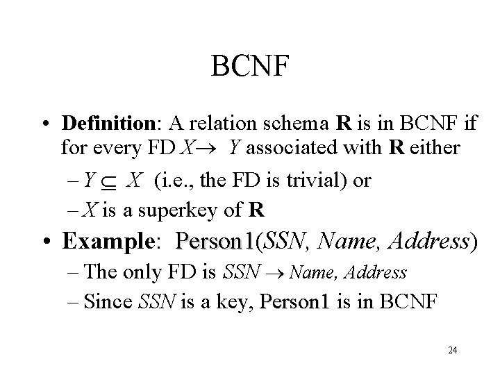
BCNF • Definition: A relation schema R is in BCNF if for every FD X Y associated with R either – Y X (i. e. , the FD is trivial) or – X is a superkey of R • Example: Person 1(SSN, Name, Address) Person 1 – The only FD is SSN Name, Address – Since SSN is a key, Person 1 is in BCNF 24

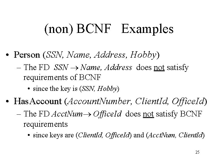
(non) BCNF Examples • Person (SSN, Name, Address, Hobby) – The FD SSN Name, Address does not satisfy requirements of BCNF • since the key is (SSN, Hobby) • Has. Account (Account. Number, Client. Id, Office. Id) – The FD Acct. Num Office. Id does not satisfy BCNF requirements • since keys are (Client. Id, Office. Id) and (Acct. Num, Client. Id) 25

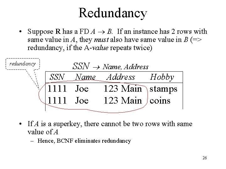
Redundancy • Suppose R has a FD A B. If an instance has 2 rows with same value in A, they must also have same value in B (=> redundancy, if the A-value repeats twice) SSN redundancy SSN Name 1111 Joe Name, Address Hobby 123 Main stamps 123 Main coins • If A is a superkey, there cannot be two rows with same value of A – Hence, BCNF eliminates redundancy 26

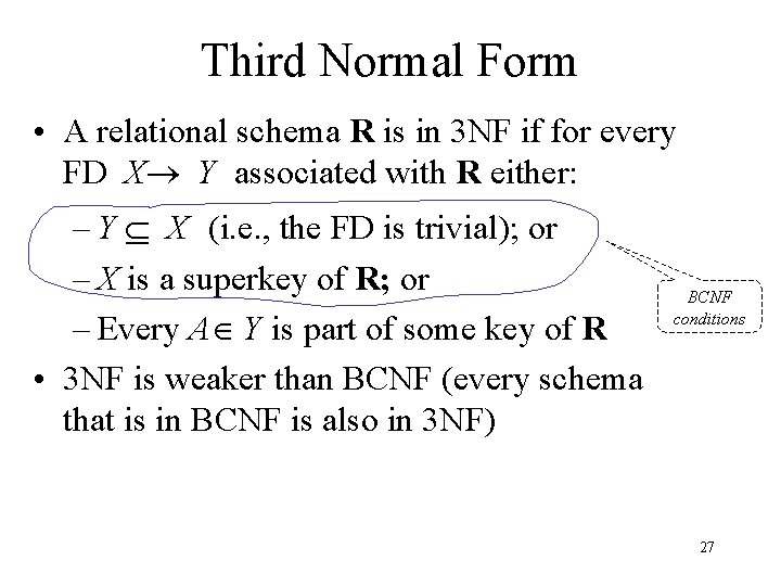
Third Normal Form • A relational schema R is in 3 NF if for every FD X Y associated with R either: – Y X (i. e. , the FD is trivial); or – X is a superkey of R; or – Every A Y is part of some key of R • 3 NF is weaker than BCNF (every schema that is in BCNF is also in 3 NF) BCNF conditions 27

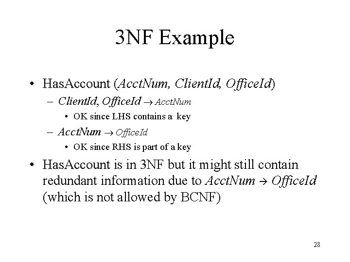
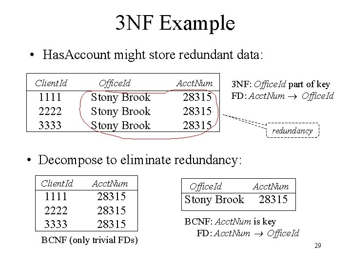
3 NF Example • Has. Account (Acct. Num, Client. Id, Office. Id) – Client. Id, Office. Id Acct. Num • OK since LHS contains a key – Acct. Num Office. Id • OK since RHS is part of a key • Has. Account is in 3 NF but it might still contain redundant information due to Acct. Num Office. Id (which is not allowed by BCNF) 28

3 NF Example • Has. Account might store redundant data: Client. Id 1111 2222 3333 Office. Id Stony Brook Acct. Num 28315 3 NF: Office. Id part of key FD: Acct. Num Office. Id redundancy • Decompose to eliminate redundancy: Client. Id Acct. Num 1111 2222 3333 28315 BCNF (only trivial FDs) Office. Id Stony Brook Acct. Num 28315 BCNF: Acct. Num is key FD: Acct. Num Office. Id 29

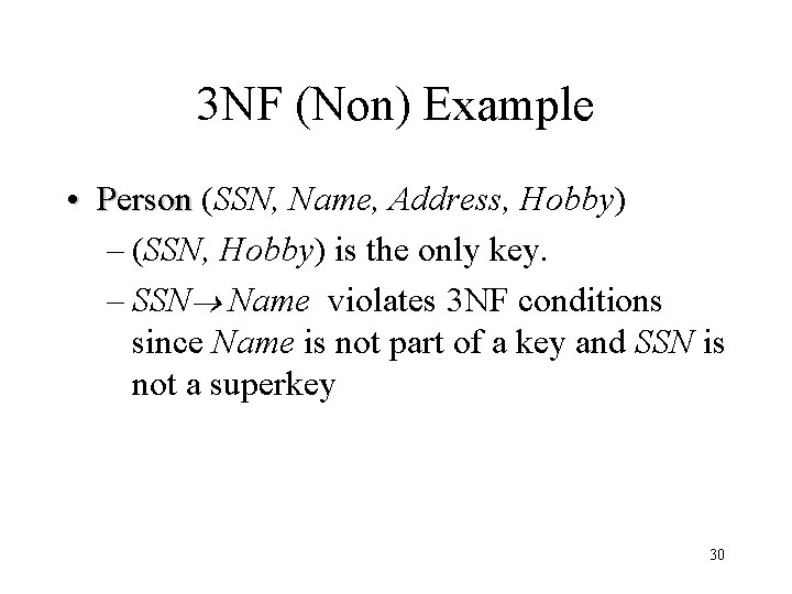
3 NF (Non) Example • Person (SSN, Name, Address, Hobby) – (SSN, Hobby) is the only key. – SSN Name violates 3 NF conditions since Name is not part of a key and SSN is not a superkey 30

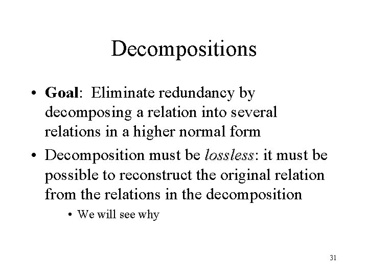
Decompositions • Goal: Eliminate redundancy by decomposing a relation into several relations in a higher normal form • Decomposition must be lossless: lossless it must be possible to reconstruct the original relation from the relations in the decomposition • We will see why 31

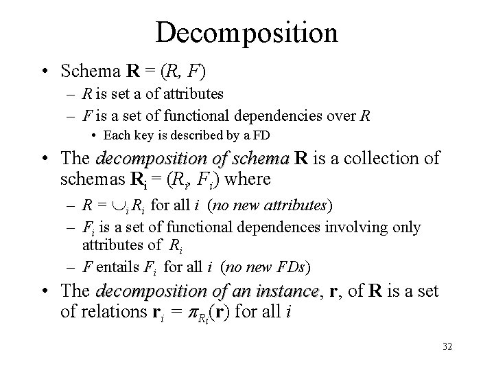
Decomposition • Schema R = (R, F) – R is set a of attributes – F is a set of functional dependencies over R • Each key is described by a FD • The decomposition of schema R is a collection of schemas Ri = (Ri, Fi) where – R = i Ri for all i (no new attributes) – Fi is a set of functional dependences involving only attributes of Ri – F entails Fi for all i (no new FDs) • The decomposition of an instance, instance r, of R is a set of relations ri = Ri(r) for all i 32

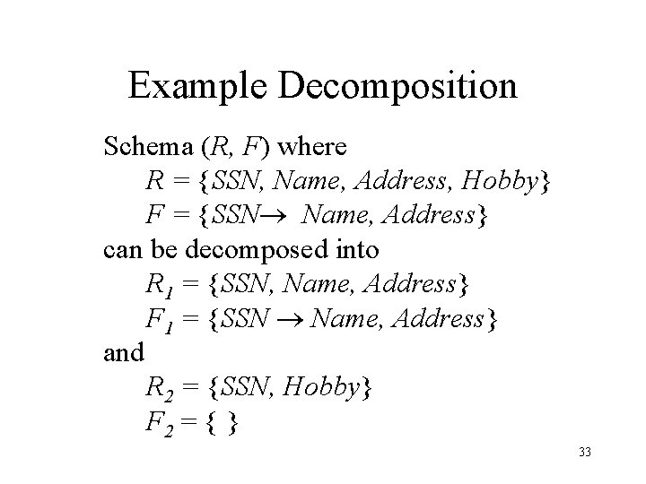
Example Decomposition Schema (R, F) where R = {SSN, Name, Address, Hobby} F = {SSN Name, Address} can be decomposed into R 1 = {SSN, Name, Address} F 1 = {SSN Name, Address} and R 2 = {SSN, Hobby} F 2 = { } 33

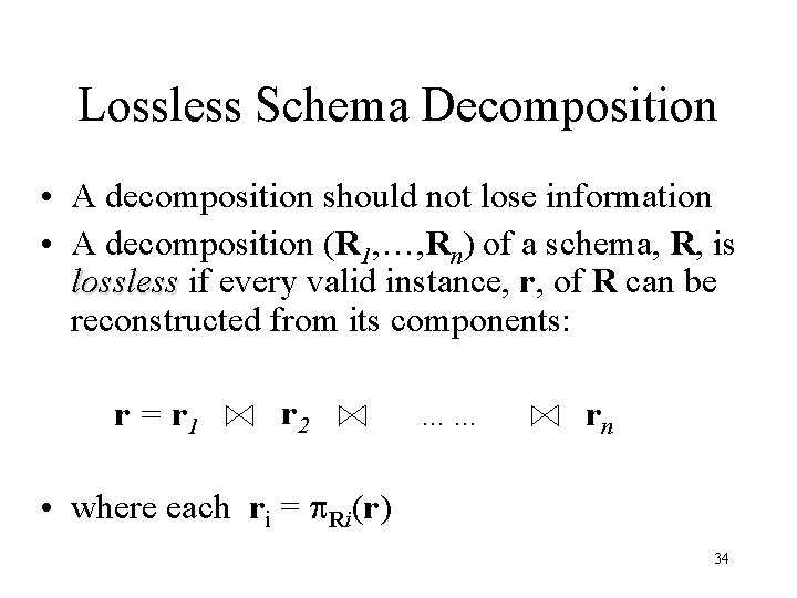
Lossless Schema Decomposition • A decomposition should not lose information • A decomposition (R 1, …, Rn) of a schema, R, is lossless if every valid instance, r, of R can be reconstructed from its components: r = r 1 r 2 …… rn • where each ri = Ri(r) 34

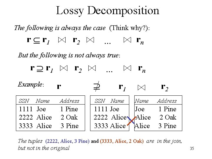
Lossy Decomposition The following is always the case (Think why? ): r r 1 r 2 rn . . . But the following is not always true: r r 1 Example: SSN Name 1111 Joe 2222 Alice 3333 Alice r 2 r rn . . . r 1 Address SSN Name 1 Pine 2 Oak 3 Pine 1111 Joe 2222 Alice 3333 Alice r 2 Name Address Joe Alice 1 Pine 2 Oak 3 Pine The tuples (2222, Alice, 3 Pine) and (3333, Alice, 2 Oak) are in the join, but not in the original 35

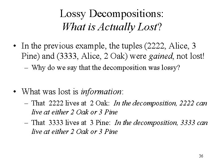
Lossy Decompositions: What is Actually Lost? • In the previous example, the tuples (2222, Alice, 3 Pine) and (3333, Alice, 2 Oak) were gained, not lost! – Why do we say that the decomposition was lossy? • What was lost is information: – That 2222 lives at 2 Oak: In the decomposition, 2222 can live at either 2 Oak or 3 Pine – That 3333 lives at 3 Pine: In the decomposition, 3333 can live at either 2 Oak or 3 Pine 36

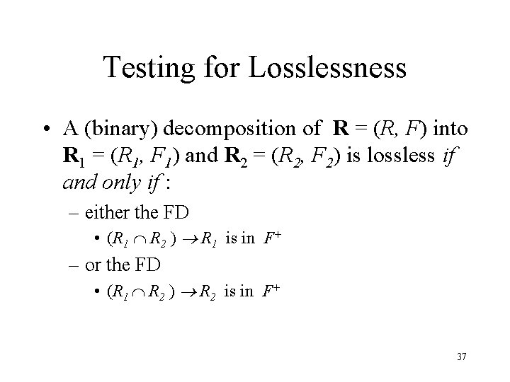
Testing for Losslessness • A (binary) decomposition of R = (R, F) into R 1 = (R 1, F 1) and R 2 = (R 2, F 2) is lossless if and only if : – either the FD • (R 1 R 2 ) R 1 is in F+ – or the FD • (R 1 R 2 ) R 2 is in F+ 37

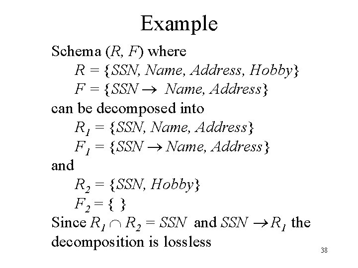
Example Schema (R, F) where R = {SSN, Name, Address, Hobby} F = {SSN Name, Address} can be decomposed into R 1 = {SSN, Name, Address} F 1 = {SSN Name, Address} and R 2 = {SSN, Hobby} F 2 = { } Since R 1 R 2 = SSN and SSN R 1 the decomposition is lossless 38

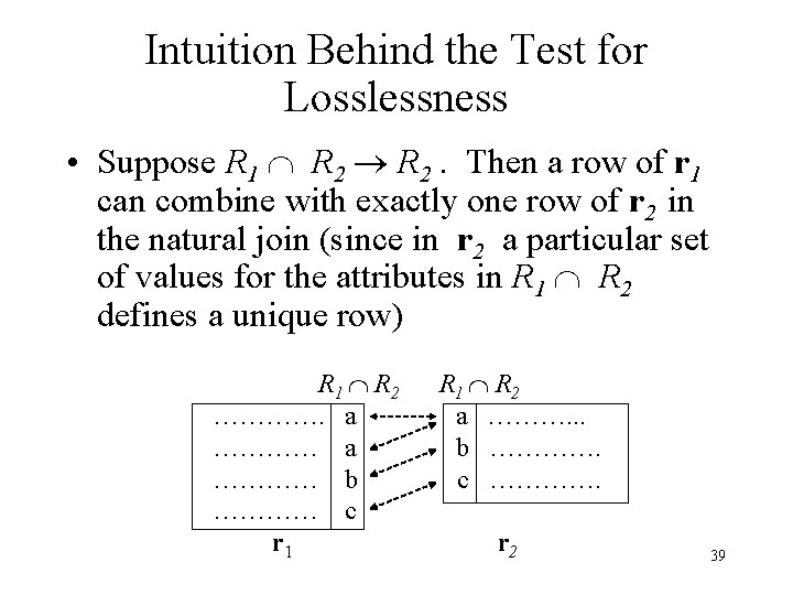
Intuition Behind the Test for Losslessness • Suppose R 1 R 2. Then a row of r 1 can combine with exactly one row of r 2 in the natural join (since in r 2 a particular set of values for the attributes in R 1 R 2 defines a unique row) R 1 R 2 …………. a ………… b ………… c r 1 R 1 R 2 a ………. . . b …………. c …………. r 2 39

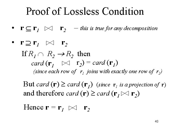
Proof of Lossless Condition • r r 1 r 2 – this is true for any decomposition r 2 • r r 1 If R 1 R 2 then r 2) = card (r 1) card (r 1 (since each row of r 1 joins with exactly one row of r 2) But card (r) card (r 1) (since r 1 is a projection of and therefore card (r) card (r 1 r 2) Hence r = r 1 r 2 40 r)

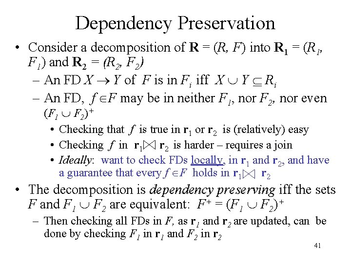
Dependency Preservation • Consider a decomposition of R = (R, F) into R 1 = (R 1, F 1) and R 2 = (R 2, F 2) – An FD X Y of F is in Fi iff X Y Ri – An FD, f F may be in neither F 1, nor F 2, nor even (F 1 F 2)+ • Checking that f is true in r 1 or r 2 is (relatively) easy • Checking f in r 1 r 2 is harder – requires a join • Ideally: want to check FDs locally, in r 1 and r 2, and have a guarantee that every f F holds in r 1 r 2 • The decomposition is dependency preserving iff the sets F and F 1 F 2 are equivalent: F+ = (F 1 F 2)+ – Then checking all FDs in F, as r 1 and r 2 are updated, can be done by checking F 1 in r 1 and F 2 in r 2 41

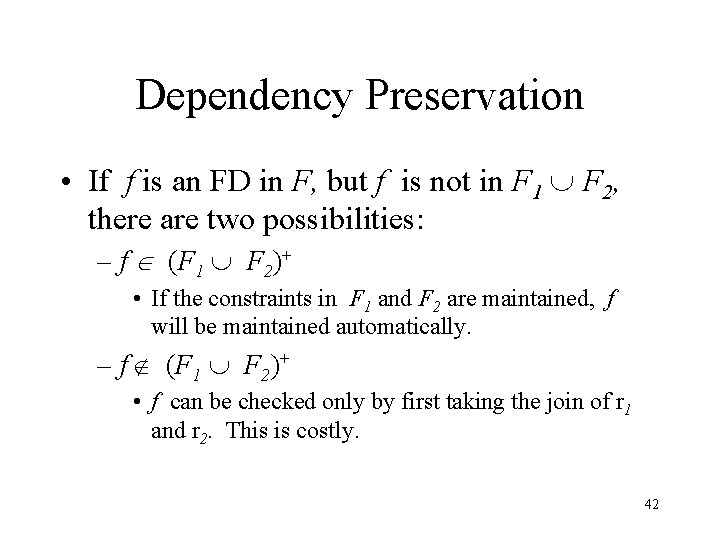
Dependency Preservation • If f is an FD in F, but f is not in F 1 F 2, there are two possibilities: – f (F 1 F 2)+ • If the constraints in F 1 and F 2 are maintained, f will be maintained automatically. – f (F 1 F 2)+ • f can be checked only by first taking the join of r 1 and r 2. This is costly. 42

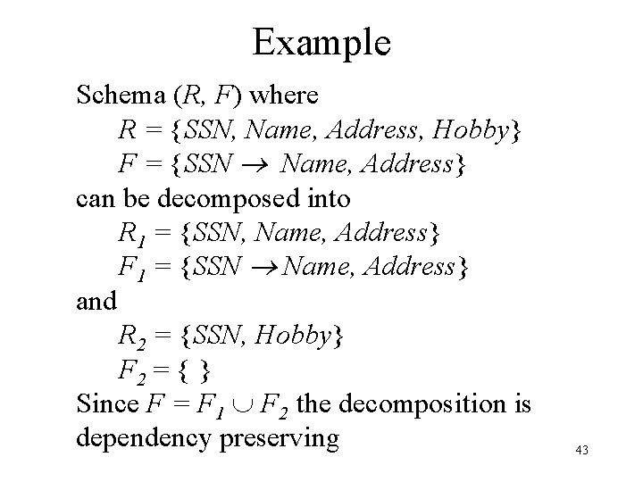
Example Schema (R, F) where R = {SSN, Name, Address, Hobby} F = {SSN Name, Address} can be decomposed into R 1 = {SSN, Name, Address} F 1 = {SSN Name, Address} and R 2 = {SSN, Hobby} F 2 = { } Since F = F 1 F 2 the decomposition is dependency preserving 43

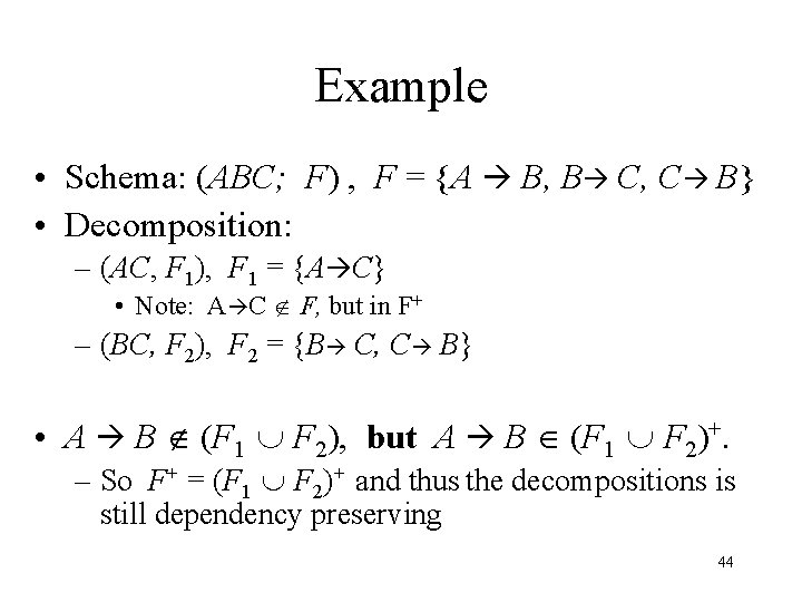
Example • Schema: (ABC; F) , F = {A B, B C, C B} • Decomposition: – (AC, F 1), F 1 = {A C} • Note: A C F, but in F+ – (BC, F 2), F 2 = {B C, C B} • A B (F 1 F 2), but A B (F 1 F 2)+. – So F+ = (F 1 F 2)+ and thus the decompositions is still dependency preserving 44

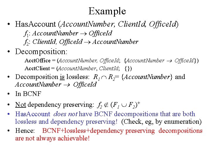
Example • Has. Account (Account. Number, Client. Id, Office. Id) f 1: Account. Number Office. Id f 2: Client. Id, Office. Id Account. Number • Decomposition: Acct. Office = (Account. Number, Office. Id; {Account. Number Office. Id}) Acct. Client = (Account. Number, Client. Id; {}) • Decomposition is lossless: R 1 R 2= {Account. Number} and Account. Number Office. Id • In BCNF • Not dependency preserving: f 2 (F 1 F 2)+ • Has. Account does not have BCNF decompositions that are both lossless and dependency preserving! (Check, eg, by enumeration) • Hence: BCNF+lossless+dependency preserving decompositions are not always achievable!

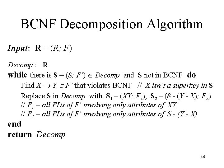
BCNF Decomposition Algorithm Input: R = (R; F) Decomp : = R while there is S = (S; F’) Decomp and S not in BCNF do Find X Y F’ that violates BCNF // X isn’t a superkey in S Replace S in Decomp with S 1 = (XY; F 1), S 2 = (S - (Y - X); F 2) // F 1 = all FDs of F’ involving only attributes of XY // F 2 = all FDs of F’ involving only attributes of S - (Y - X) end return Decomp 46

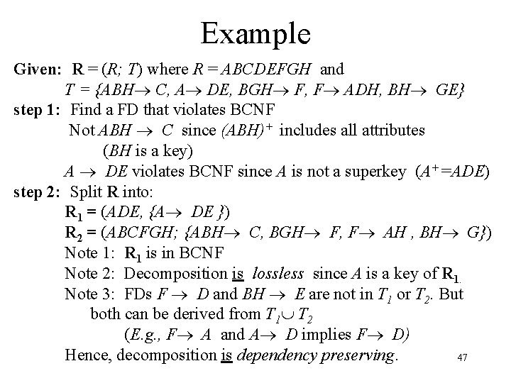
Example Given: R = (R; T) where R = ABCDEFGH and T = {ABH C, A DE, BGH F, F ADH, BH GE} step 1: Find a FD that violates BCNF Not ABH C since (ABH)+ includes all attributes (BH is a key) A DE violates BCNF since A is not a superkey (A+ =ADE) step 2: Split R into: R 1 = (ADE, {A DE }) R 2 = (ABCFGH; {ABH C, BGH F, F AH , BH G}) Note 1: R 1 is in BCNF Note 2: Decomposition is lossless since A is a key of R 1. Note 3: FDs F D and BH E are not in T 1 or T 2. But both can be derived from T 1 T 2 (E. g. , F A and A D implies F D) Hence, decomposition is dependency preserving. 47

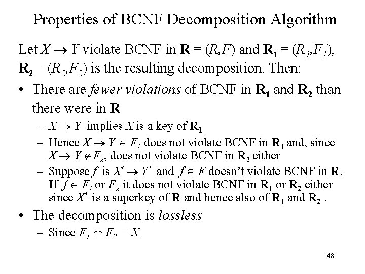
Properties of BCNF Decomposition Algorithm Let X Y violate BCNF in R = (R, F) and R 1 = (R 1, F 1), R 2 = (R 2, F 2) is the resulting decomposition. Then: • There are fewer violations of BCNF in R 1 and R 2 than there were in R – X Y implies X is a key of R 1 – Hence X Y F 1 does not violate BCNF in R 1 and, since X Y F 2, does not violate BCNF in R 2 either – Suppose f is X’ Y’ and f F doesn’t violate BCNF in R. If f F 1 or F 2 it does not violate BCNF in R 1 or R 2 either since X’ is a superkey of R and hence also of R 1 and R 2. • The decomposition is lossless – Since F 1 F 2 = X 48

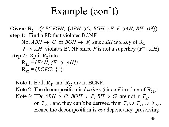
Example (con’t) Given: R 2 = (ABCFGH; {ABH C, BGH F, F AH, BH G}) step 1: Find a FD that violates BCNF. Not ABH C or BGH F, since BH is a key of R 2 F AH violates BCNF since F is not a superkey (F+ =AH) step 2: Split R 2 into: R 21 = (FAH, {F AH}) R 22 = (BCFG; {}) Note 1: Both R 21 and R 22 are in BCNF. Note 2: The decomposition is lossless (since F is a key of R 21) Note 3: FDs ABH C, BGH F, BH G are not in T 21 or T 22 , and they can’t be derived from T 1 T 22. Hence the decomposition is not dependency-preserving 49

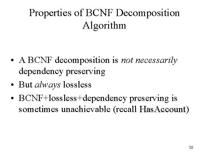
Properties of BCNF Decomposition Algorithm • A BCNF decomposition is not necessarily dependency preserving • But always lossless • BCNF+lossless+dependency preserving is sometimes unachievable (recall Has. Account) Has. Account 50

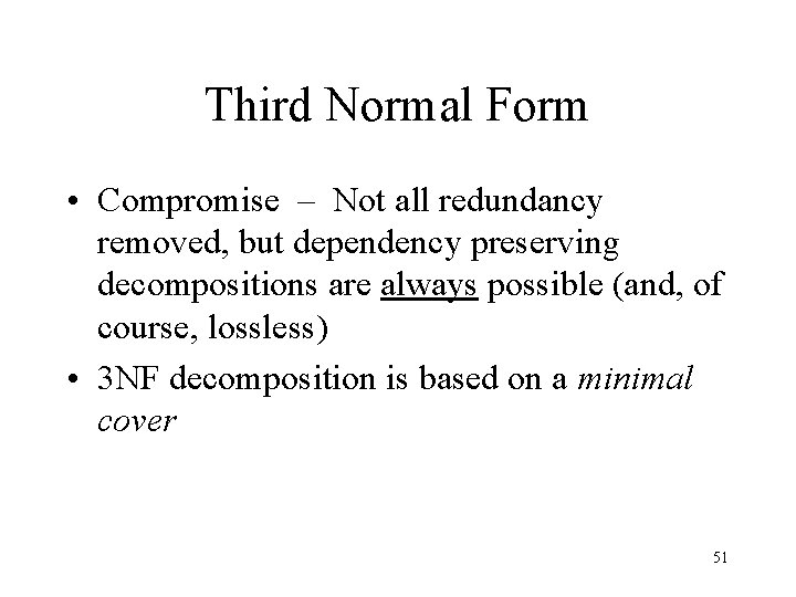
Third Normal Form • Compromise – Not all redundancy removed, but dependency preserving decompositions are always possible (and, of course, lossless) • 3 NF decomposition is based on a minimal cover 51

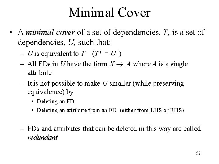
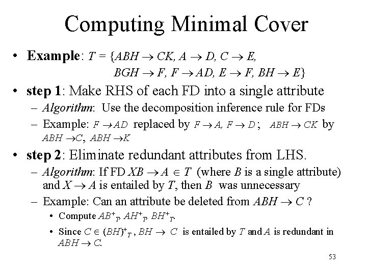
Minimal Cover • A minimal cover of a set of dependencies, T, is a set of dependencies, U, such that: – U is equivalent to T (T+ = U+) – All FDs in U have the form X A where A is a single attribute – It is not possible to make U smaller (while preserving equivalence) by • Deleting an FD • Deleting an attribute from an FD (either from LHS or RHS) – FDs and attributes that can be deleted in this way are called redundant 52

Computing Minimal Cover • Example: T = {ABH CK, A D, C E, BGH F, F AD, E F, BH E} • step 1: Make RHS of each FD into a single attribute – Algorithm: Use the decomposition inference rule for FDs – Example: F AD replaced by F A, F D ; ABH CK by ABH C, ABH K • step 2: Eliminate redundant attributes from LHS. – Algorithm: If FD XB A T (where B is a single attribute) and X A is entailed by T, then B was unnecessary – Example: Can an attribute be deleted from ABH C ? • Compute AB+T, AH+T, BH+T. • Since C (BH)+T , BH C is entailed by T and A is redundant in ABH C. 53

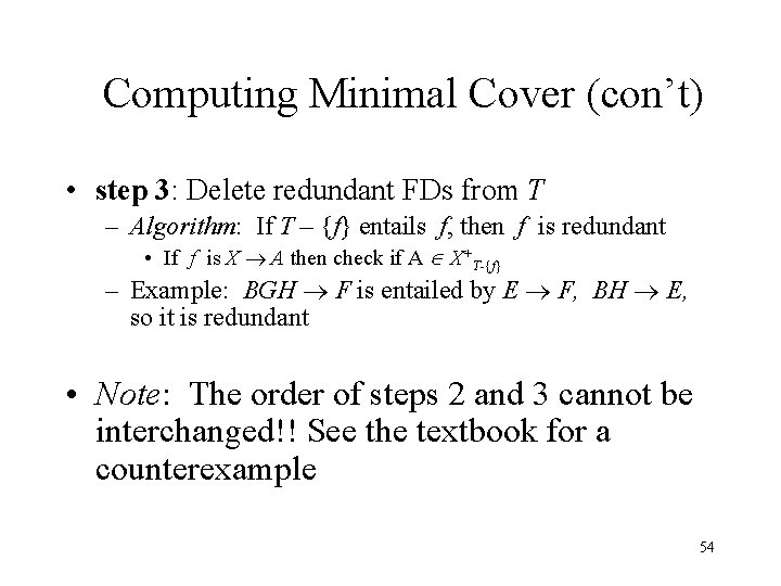
Computing Minimal Cover (con’t) • step 3: Delete redundant FDs from T – Algorithm: If T – {f} entails f, then f is redundant • If f is X A then check if A X+T-{f} – Example: BGH F is entailed by E F, BH E, so it is redundant • Note: The order of steps 2 and 3 cannot be interchanged!! See the textbook for a counterexample 54

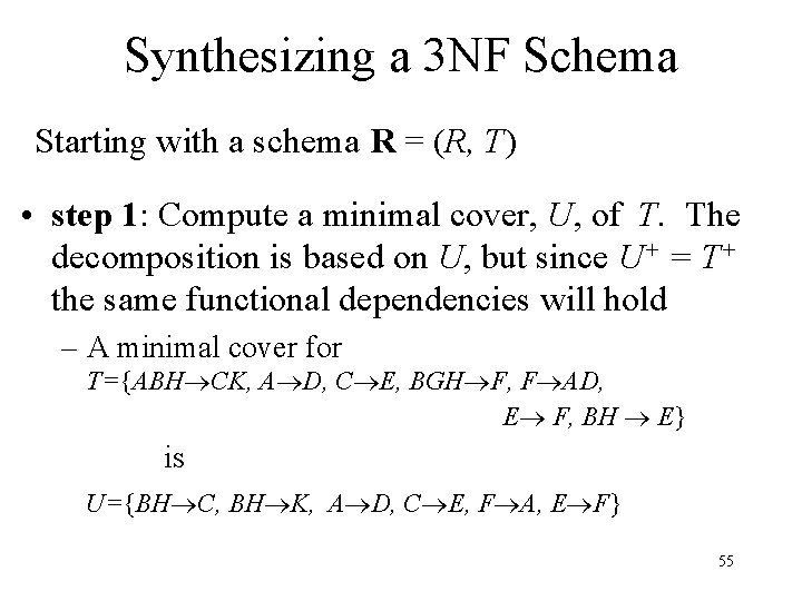
Synthesizing a 3 NF Schema Starting with a schema R = (R, T) • step 1: Compute a minimal cover, U, of T. The decomposition is based on U, but since U+ = T+ the same functional dependencies will hold – A minimal cover for T={ABH CK, A D, C E, BGH F, F AD, E F, BH E} is U={BH C, BH K, A D, C E, F A, E F} 55

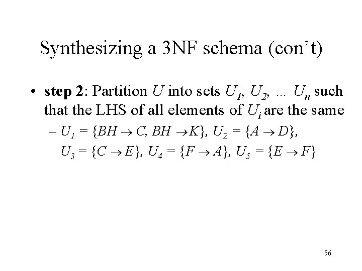
Synthesizing a 3 NF schema (con’t) • step 2: Partition U into sets U 1, U 2, … Un such that the LHS of all elements of Ui are the same – U 1 = {BH C, BH K}, U 2 = {A D}, U 3 = {C E}, U 4 = {F A}, U 5 = {E F} 56

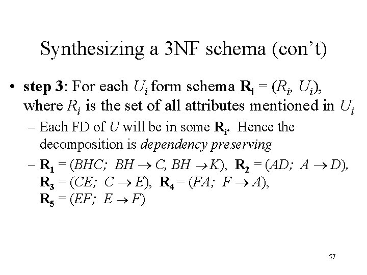
Synthesizing a 3 NF schema (con’t) • step 3: For each Ui form schema Ri = (Ri, Ui), where Ri is the set of all attributes mentioned in Ui – Each FD of U will be in some Ri. Hence the decomposition is dependency preserving – R 1 = (BHC; BH C, BH K), R 2 = (AD; A D), R 3 = (CE; C E), R 4 = (FA; F A), R 5 = (EF; E F) 57

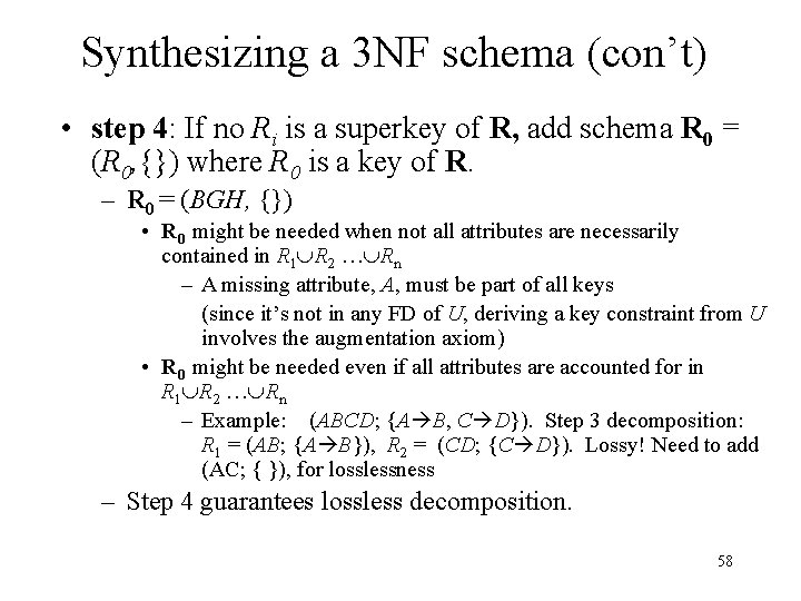
Synthesizing a 3 NF schema (con’t) • step 4: If no Ri is a superkey of R, add schema R 0 = (R 0, {}) where R 0 is a key of R. – R 0 = (BGH, {}) • R 0 might be needed when not all attributes are necessarily contained in R 1 R 2 … Rn – A missing attribute, A, must be part of all keys (since it’s not in any FD of U, deriving a key constraint from U involves the augmentation axiom) • R 0 might be needed even if all attributes are accounted for in R 1 R 2 … Rn – Example: (ABCD; {A B, C D}). Step 3 decomposition: R 1 = (AB; {A B}), R 2 = (CD; {C D}). Lossy! Need to add (AC; { }), for losslessness – Step 4 guarantees lossless decomposition. 58

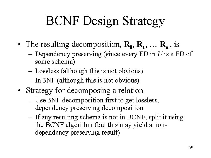
BCNF Design Strategy • The resulting decomposition, R 0, R 1, … Rn , is – Dependency preserving (since every FD in U is a FD of some schema) – Lossless (although this is not obvious) – In 3 NF (although this is not obvious) • Strategy for decomposing a relation – Use 3 NF decomposition first to get lossless, dependency preserving decomposition – If any resulting schema is not in BCNF, split it using the BCNF algorithm (but this may yield a nondependency preserving result) 59

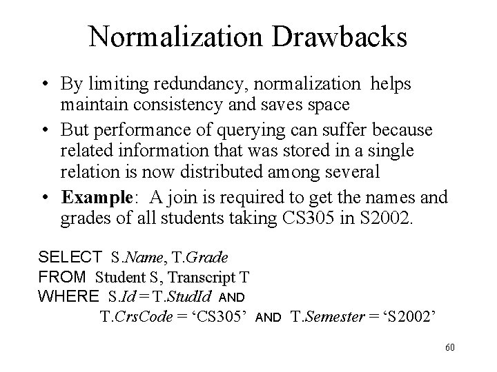
Normalization Drawbacks • By limiting redundancy, normalization helps maintain consistency and saves space • But performance of querying can suffer because related information that was stored in a single relation is now distributed among several • Example: A join is required to get the names and grades of all students taking CS 305 in S 2002. SELECT S. Name, T. Grade FROM Student S, Transcript T WHERE S. Id = T. Stud. Id AND T. Crs. Code = ‘CS 305’ AND T. Semester = ‘S 2002’ 60

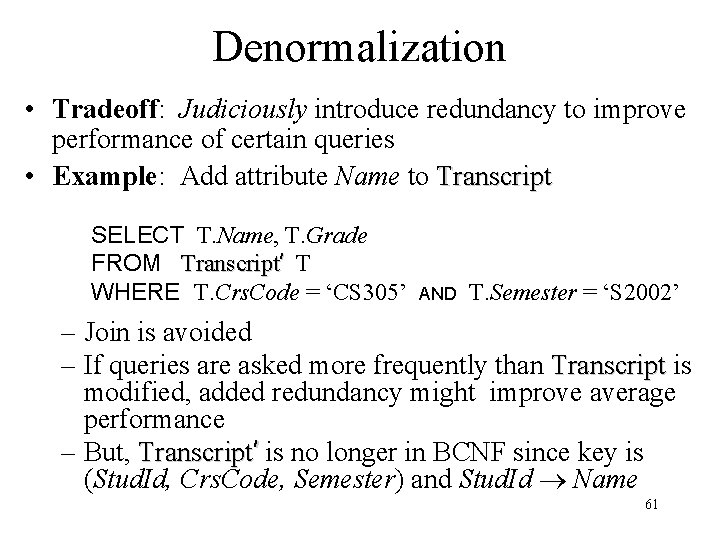
Denormalization • Tradeoff: Judiciously introduce redundancy to improve performance of certain queries • Example: Add attribute Name to Transcript SELECT T. Name, T. Grade FROM Transcript’ T WHERE T. Crs. Code = ‘CS 305’ AND T. Semester = ‘S 2002’ – Join is avoided – If queries are asked more frequently than Transcript is modified, added redundancy might improve average performance – But, Transcript’ is no longer in BCNF since key is (Stud. Id, Crs. Code, Semester) and Stud. Id Name 61

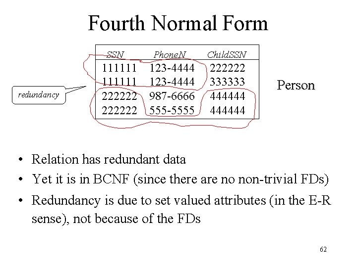
Fourth Normal Form SSN redundancy 111111 222222 Phone. N 123 -4444 987 -6666 555 -5555 Child. SSN 222222 333333 444444 Person • Relation has redundant data • Yet it is in BCNF (since there are no non-trivial FDs) • Redundancy is due to set valued attributes (in the E-R sense), not because of the FDs 62

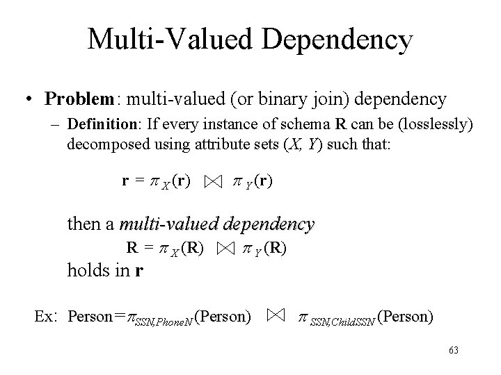
Multi-Valued Dependency • Problem: multi-valued (or binary join) dependency – Definition: If every instance of schema R can be (losslessly) decomposed using attribute sets (X, Y) such that: r = X (r) Y (r) then a multi-valued dependency R = X (R) holds in r Y (R) Ex: Person= SSN, Phone. N (Person) Person SSN, Child. SSN (Person) Person 63

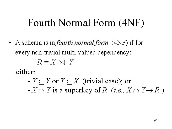
Fourth Normal Form (4 NF) • A schema is in fourth normal form (4 NF) if for every non-trivial multi-valued dependency: R=X Y either: - X Y or Y X (trivial case); or - X Y is a superkey of R (i. e. , X Y R ) 64

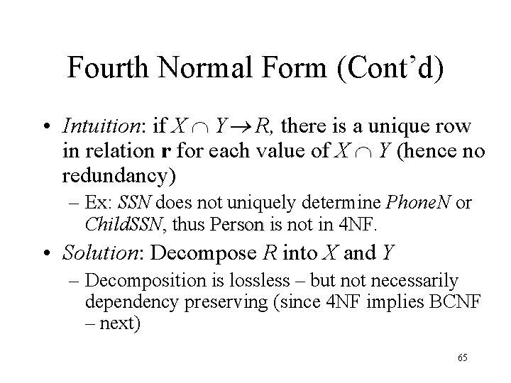
Fourth Normal Form (Cont’d) • Intuition: if X Y R, there is a unique row in relation r for each value of X Y (hence no redundancy) – Ex: SSN does not uniquely determine Phone. N or Child. SSN, thus Person is not in 4 NF. • Solution: Decompose R into X and Y – Decomposition is lossless – but not necessarily dependency preserving (since 4 NF implies BCNF – next) 65

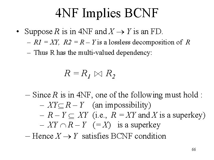
4 NF Implies BCNF • Suppose R is in 4 NF and X Y is an FD. – R 1 = XY, R 2 = R – Y is a lossless decomposition of R – Thus R has the multi-valued dependency: R = R 1 R 2 – Since R is in 4 NF, one of the following must hold : – XY R – Y (an impossibility) – R – Y XY (i. e. , R = XY and X is a superkey) – XY R – Y (= X) is a superkey – Hence X Y satisfies BCNF condition 66