DATA TRANSFORMATION and NORMALIZATION Lecture Topic 4 DATA

DATA TRANSFORMATION and NORMALIZATION Lecture Topic 4

DATA PRE-PROCESSING • TRANSFORMATION • NORMALIZATION • SCALING

DATA TRANSFORMATION • Difference between raw fluorescence is a meaningless number • Data is transformed: – Ratio allows immediate visualization of number – Log

Why Log 2? • Difference in expression intensity exist on a multiplicative scale, log transformation brings them into the additive scale, where a linear model may apply. • • • Ex. 4 fold repression=0. 25 (Log 2=-2) Ex. 4 fold induction=4 ( Log 2=2) Ex. 16 fold induction=16 (Log 2= 4) Ex. 16 fold repression=0. 0625 (Log 2=-4) Evens out highly skewed distributions Makes variation of intensities…independent of absolute magnitude

Log Transformation: Makes the distribution less skewed

Example 2

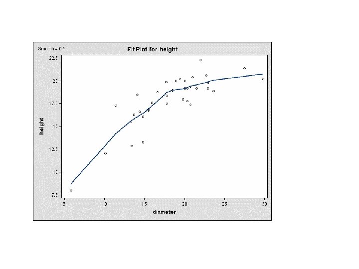
Non-parametric Regression: the Loess Method • LOWESS= LOESS is an Acronym for LOcally re. WEighted Scatter. Plot Smoothing (Cleveland). • For i=1 to n, the ith measurement yi of the response y and the corresponding measurement xi of the vector x of p predictors are related by • Yi=g(xi) + e. I • where g is the regression function and ei is a random error. • Idea: g(x) can be locally approximated by a parametric function. • Obtained by fitting a regression surface to the data points within a chosen neighborhood of the point x.

LOESS contd… • In the LOESS (LOWESS) method, weighted least squares is used to fit linear or quadratic functions of the predictors at the centers of neighborhoods. • The radius of each neighborhood is chosen so that the neighborhood contains a specified percentage of the data points. The fraction of the data, called the smoothing parameter, in each local neighborhood controls the smoothness of the estimated surface. • Data points in a given local neighborhood are weighted by a smooth decreasing function of their distance from the center of the neighborhood.

Distance metrics used • Finding distance between the ith and hth points 2 predictors: • Distance between: (Xi 1, Xi 2) and (Xh 1, Xh 2): • Generally Eucledean Distance is used, • and weights are defined by a tri-cube function: • Choice of q is between 0 and 1, often between. 4 to. 6. • Large q: smoother but maybe too smooth • Small q: too rough

Comments on LOESS · fitting is done at each point at which the regression surface is to be estimated · faster computational procedure is to perform such local fitting at a selected sample of points and then to blend local polynomials to obtain a regression surface · can use the LOESS procedure to perform statistical inference provided the error distribution are i. i. d. normal random variables with mean 0. · using the iterative reweighting, LOESS can also provide statistical inference when the error distribution is symmetric but not necessarily normal. · by doing iterative reweighting, you can use the LOESS procedure to perform robust fitting in the presence of outliers in the data.

Data “Normalization” • To biologists, data normalization means “eliminating systematic noise” from the data • Noise is systematic variation – experimental variation, human error, variation of scanner technology, etc • Variation in which we are NOT interested • We are interested in measuring true biologic variation of genes across experiments, throughout time, etc. • Plays an important role in earlier stages of microarray data analysis. • Subsequent analysis are highly dependent on normalization. • NORMALIZATION: Adjusts from any bias which arises from microarray technology rather than biological

Normalization: Age old Statistical Idea • • Stands for removing bias as a result of experimental artifacts from the data. Stems back to Fisher’s idea (1923) setting up of ANOVA. There is a thrust to use ANOVA for normalization, but for the most part it is still a stage-wise approach instead of a model taking out all sources of variation at once. We will need to look at: – – – Spatial correction Background correction Dye-effect correction Within replicate rescaling Across replicate rescaling • Within slide normalization • Paired slide normalization for dye swap • Multiple slide normalization

M vs A plots • Used to look at agreement of variables intended to measure the same response. • • • Consider y 1 and y 2 measure the same variable (two reps of the same variable) M or Minus = (y 1 -y 2) A or Average = (y 1+y 2)/2 • Often done in the log scale (M=log(y 1/y 2) A= log((y 1*y 2)/2) • If we plot M on the y-axis and A on the X axis, we expect to see a flat line, if the two variables do indeed measure the same thing.

Code ma. data=read. csv("MA. csv", header=TRUE) head(ma. data) y 1=ma. data$slide 1 y 2=ma. data$slide 2 M=y 1 -y 2 A=(y 1+y 2)/2 plot(y 1, y 2) plot(A, M) lw 1 <- loess(M ~ A, data=ma. data, span=0. 10) plot(M ~ A, data=ma. data) j <- order(A) lines(A[j], lw 1$fitted[j], col="red", lwd=3) #idea of normalization fit=lw 1$fitted new. M=M-fit lw 2 <- loess(new. M ~ A, data=ma. data, span=0. 10) plot(new. M ~ A, data=ma. data) j <- order(A) lines(A[j], lw 2$fitted[j], col=“green", lwd=3) #plotting all on the same plot(M ~ A, data=ma. data) lines(A[j], lw 1$fitted[j], col="red", lwd=3) lines(A[j], lw 2$fitted[j], col="green", lwd=3)

Array 1: pre and post norm

Comments: • Print-tip normalization is generally a good proxy for spatial effects • Instead of LOESS one can use SPLINE to estimate the trend to subtract from the raw data.

BACKGROUND CORRECTION • Idea: • Signal = True Signal + Background • So, an attractive idea seems like we should subtract BACKGROUND from the signal to get to the “TRUE” signal. • The problem is that, the actual BACKGROUND in a spot cannot be measured and what is measured are really a “estimate” for background of places NEAR the spot. • Criticism: the assumption in these models is that the background is additive – OFTEN WE SEE HIGN CORRELATION BETWEEN FOREGROUND AND BACKGROUND. – GENERAL CONSENSUS THESE DAYS: NOT TO SUBTRACT LOCAL BACKGROUND, BUT POSSIBLY SUBTRACT A GLOBAL BACKGROUND (FROM EMPTY SPOTS OR BUFFERS).

Background Correction: more thoughts • Mc. Clure and Wit (2004) suggest calculating the mean or median of the empty spots and estimate, signal as: – Signal = max(observed signal – center(empty spots), 0) This allows never to have the problem of negative “corrected signals”.

Background Correction: Probabilistic Idea • Irrizary et al(2003) • Looks at finding the conditional expectation of the TRUE signal given the observed signal (which is assumed to be the true signal plus noise) • E(si | si+bi) • Here, si assumed to follow Exponential distribution with parameter q. • Bi assumed to follow N(me, s 2 e) • Estimate me and se as the mean and standard deviation of empty spots

Normalization Approaches • GLOBAL Normalization (G): Global (ARRAY) Mean or Median. – NOT USED VERY OFTEN ANYMORE • Intensity dependent linear Normalization (L): by least square estimation – AGAIN NOT USED AS MUCH • Intensity dependent non-linear Normalization (N): Lowess curve (Robust scatter plot smoother) – Under ideal experimental conditions: M=0 for the selected genes used for normalization – THE MOST COMMONLY USED IDEA THESE DAYS.

Normalization: Historical Approaches • Gobal normalization – Sum method: Norm coef. (kj) = Where Imi = intensity of gene i on array Array m, m=1, 2 Bm= background intensity on Array m, m=1, 2 n = number of genes on the array – problem: validity of the assumption; stronger signals dominate the summation. – Median (robust with respect to outliers) Normalization coefficient (kj) =

Normalization continued • Housekeeping gene normalization – Housekeeping genes are a set of genes whose expression levels are not affected by the treatment. – The normalization coefficient is the ratio of m. C/m. T, where m. C and m. T are the means of the selected housekeeping genes for control and treatment respectively. – Problem: housekeeping genes change their expression level sometimes. The assumption doesn’t hold. • Trimmed mean normalization(adjusted global method) trim off 5% highest and lowest extreme values, then globally normalize data. The normalization coefficient is: where are the trimmed means for the ith treatment and control respectively.

Ideal Control Spots that should be on an array As we saw in the previous slide, there can be many special probes spotted onto an array during its manufacture, collectively called control probes. These include • Blanks: places where water or nothing is spotted. • Buffer: where the buffer solution without DNA is spotted. • Negative: here there are DNA probes, but they shouldn’t be complementary to any target c. DNA. • Calibration: probes corresponding to DNA put in the hyb mix which should have equal signals in the two channels. • Ratio: probes corresponding to DNA put in the hyb mix which should have known ratios between the two channels (e. g. 3: 1, 1: 3, 10: 1, 1: 10).

Normalization Within and Across Conditions • The Normalization WITHIN conditions is more common • Idea we want all the arrays that represent the SAME condition to be comparable. • Take out the array effect, in other words. • Many models for this: – Factorial model (Kerr et al, Wolfinger et al) – Location Scale Model (Yang et al) – Scaling (Affymetrix) Consider the data to be: xijk: ith spot, jth color, kth array

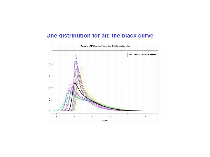
Quantile Normalization Idea • Ideally “replicate” microarrays should be similar • In real life they are often NOT identically distributed • Quantile normalization FORCES the same distribution on all the arrays for the same condition

Mathematical details: Quantile Normalization • {x} represent the matrix of all p spot intensities and the n replicate arrays. • Here, xik is the spot intensity of the ith spot (i=1, …p, k=1, …n). • Let x(k) = vector of the smallest spot intensities across the arrays • be the mean/median of x(j) • The vector represents the compromise distribution. {r} be the matrix of row ranks associated with matrix {x} • Then, the following are the quantile normalized value

Numerical Example • Let us consider a situation where we have 5 spots on an array and two replicates for an array (numbers in brackets represents the ranks) • Spot 1 2 3 4 5 • Array 1 16(5) 0(1) 9(3) 11(4) 7(2) • Array 2 13(4) 3(1) 5(2) 14(5) 8(3) • Order the arrays: 0 7 9 11 16 • Array 2 3 5 8 13 14 • Average these: 1. 5 6 8. 5 12 15 • Replace the ranks by these: • Normalized arrays are: • Array 1: 15 1. 5 8. 5 12 6. 0 • Array 2: 12 1. 5 6. 0 15 8. 5

R code #need to install files from Bioconductor #For R version 3. 6 onwards we need to do the following: if (!require. Namespace("Bioc. Manager", quietly = TRUE)) install. packages("Bioc. Manager") Bioc. Manager: : install(c("Genomic. Features", "Annotation. Dbi")) Bioc. Manager: : install("affy") Bioc. Manager: : install("affy. PLM") library(affy. PLM) #load package library(preprocess. Core) #create a matrix using the same example mat 1=matrix(c(16, 0, 9, 11, 7, 13, 3, 5, 14, 8), ncol=2) normalize. quantiles(mat 1)

Conclusion • No unique normalization method for the same data. It depends on what kind of experiment you have and what the data look like. • No absolute criteria for normalization. Basically, the normalized log ratio should be centered around 0. • Nowadays the focus IS on using Nonparametric Regression methods to remove trend or spatial artifacts from the data • Quantile normalization (though not liked by BIOLOGISTS) is catching on as well.