Normalization and Data Mining RG Chapter 19 Lecture

Normalization and Data Mining R&G Chapter 19 Lecture 27 Science is the knowledge of consequences, and dependence of one fact upon another. Thomas Hobbes (1588 -1679)

Administrivia • Homework Due a week from Today – Ruby. On. Rails help session Wed, 5 -7 pm, 310 Soda – (Thanks to Darren Lo & HKN) • Final exam 3 weeks from tomorrow

Review: Functional Dependencies – – Properties of the real world Decide when to decompose relations Help us find keys Help us evaluate Design Tradeoffs • Want to reduce redundancy, avoid anomalies • Want reasonable efficiency • Must avoid lossy decompositions – F+: closure, all dependencies that can be inferred from a set F – A+: attribute closure, all attributes functionally determined by the set of attributes A – G: minimal cover, smallest set of FDs such that G+ == F+

Review: Normal Forms • A property of a single relation • Tells us something about redundancy in reln • Reln R with FDs F is in BCNF if, for all X A in F+ A X (called a trivial FD), or X is a superkey for R. • Reln R with FDs F is in 3 NF if, for all X A in F+ A X (called a trivial FD), or X is a superkey of R, or A is part of some candidate key (not superkey!) for R. (sometimes stated as “A is prime”)

Review: Decomposition • If reln violates normal form, decompose – but must have lossless decomposition • Lossless decomposition: – decomposition of R into X and Y is lossless if and only if X Y is a key for either X or Y – If W Z holds over R and (W Z) is empty, then decomposition of R into R-Z and WZ is loss-less. • Algorithm: – For each FD W Z in R that violates normal form, decompose R into R-Z and WZ. Repeat as needed. – Order not important, but can produce very different results

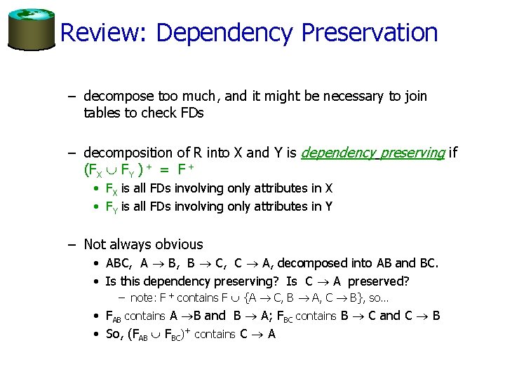
Review: Dependency Preservation – decompose too much, and it might be necessary to join tables to check FDs – decomposition of R into X and Y is dependency preserving if (FX FY ) + = F + • FX is all FDs involving only attributes in X • FY is all FDs involving only attributes in Y – Not always obvious • ABC, A B, B C, C A, decomposed into AB and BC. • Is this dependency preserving? Is C A preserved? – note: F + contains F {A C, B A, C B}, so… • FAB contains A B and B A; FBC contains B C and C B • So, (FAB FBC)+ contains C A

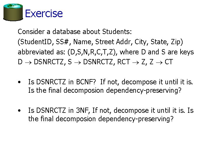
Exercise Consider a database about Students: (Student. ID, SS#, Name, Street Addr, City, State, Zip) abbreviated as: (D, S, N, R, C, T, Z), where D and S are keys D DSNRCTZ, S DSNRCTZ, RCT Z, Z CT • Is DSNRCTZ in BCNF? If not, decompose it until it is. Is the final decomposion dependency-preserving? • Is DSNRCTZ in 3 NF, If not, decompose it until it is. Is the final decomposion dependency-preserving?

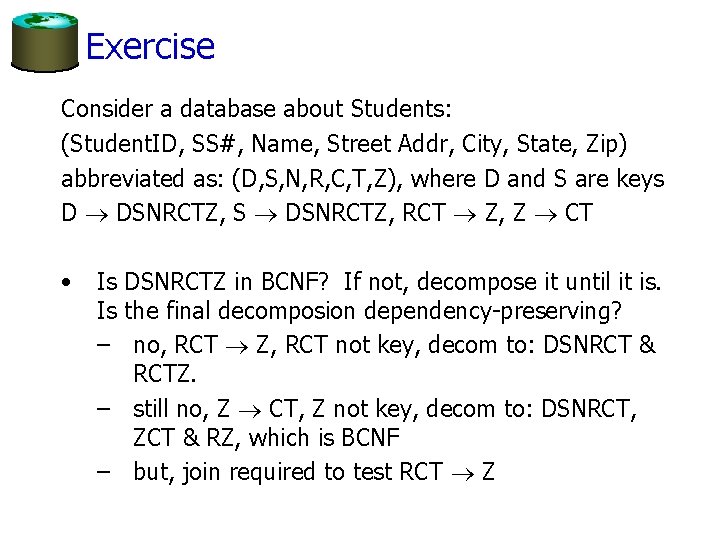
Exercise Consider a database about Students: (Student. ID, SS#, Name, Street Addr, City, State, Zip) abbreviated as: (D, S, N, R, C, T, Z), where D and S are keys D DSNRCTZ, S DSNRCTZ, RCT Z, Z CT • Is DSNRCTZ in BCNF? If not, decompose it until it is. Is the final decomposion dependency-preserving? – no, RCT Z, RCT not key, decom to: DSNRCT & RCTZ. – still no, Z CT, Z not key, decom to: DSNRCT, ZCT & RZ, which is BCNF – but, join required to test RCT Z

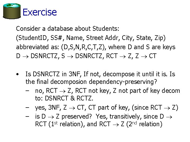
Exercise Consider a database about Students: (Student. ID, SS#, Name, Street Addr, City, State, Zip) abbreviated as: (D, S, N, R, C, T, Z), where D and S are keys D DSNRCTZ, S DSNRCTZ, RCT Z, Z CT • Is DSNRCTZ in 3 NF, If not, decompose it until it is. Is the final decomposion dependency-preserving? – no, RCT Z, RCT not key, Z not part of key decom to: DSNRCT & RCTZ. – yes, 3 NF, Z CT, CT part of key, (since RCT Z) – is D Z preserved? Yes, transitively, since D RCT (1 st relation), and RCT Z (2 nd relation)

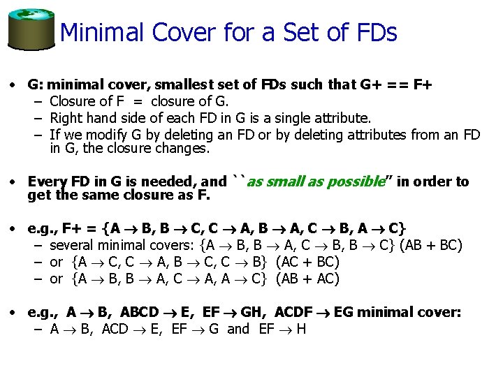
Minimal Cover for a Set of FDs • G: minimal cover, smallest set of FDs such that G+ == F+ – Closure of F = closure of G. – Right hand side of each FD in G is a single attribute. – If we modify G by deleting an FD or by deleting attributes from an FD in G, the closure changes. • Every FD in G is needed, and ``as small as possible’’ in order to get the same closure as F. • e. g. , F+ = {A B, B C, C A, B A, C B, A C} – several minimal covers: {A B, B A, C B, B C} (AB + BC) – or {A C, C A, B C, C B} (AC + BC) – or {A B, B A, C A, A C} (AB + AC) • e. g. , A B, ABCD E, EF GH, ACDF EG minimal cover: – A B, ACD E, EF G and EF H

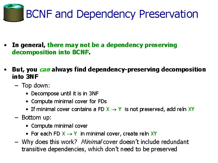
BCNF and Dependency Preservation • In general, there may not be a dependency preserving decomposition into BCNF. • But, you can always find dependency-preserving decomposition into 3 NF – Top down: • Decompose until it is in 3 NF • Compute minimal cover for FDs • If minimal cover contains a FD X Y is not preserved, add reln XY – Bottom up: • Compute minimal cover • For each FD X Y in minimal cover, create reln XY – Why does this work? Minimal cover doesn’t include redundant transitive dependencies, which don’t need to be preserved

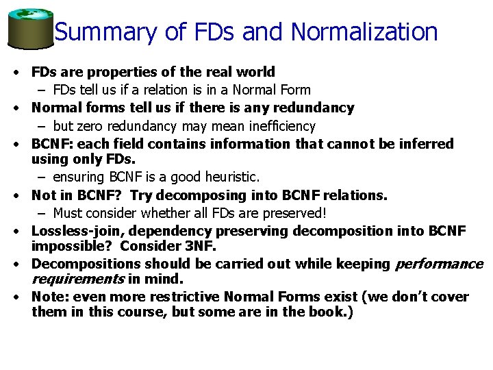
Summary of FDs and Normalization • FDs are properties of the real world – FDs tell us if a relation is in a Normal Form • Normal forms tell us if there is any redundancy – but zero redundancy may mean inefficiency • BCNF: each field contains information that cannot be inferred using only FDs. – ensuring BCNF is a good heuristic. • Not in BCNF? Try decomposing into BCNF relations. – Must consider whether all FDs are preserved! • Lossless-join, dependency preserving decomposition into BCNF impossible? Consider 3 NF. • Decompositions should be carried out while keeping performance requirements in mind. • Note: even more restrictive Normal Forms exist (we don’t cover them in this course, but some are in the book. )

New Topic: Data Mining

Definition Data mining is the exploration and analysis of large quantities of data in order to discover valid, novel, potentially useful, and ultimately understandable patterns in data. Example pattern (Census Bureau Data): If (relationship = husband), then (gender = male). 99. 6%

Definition (Cont. ) Data mining is the exploration and analysis of large quantities of data in order to discover valid, novel, potentially useful, and ultimately understandable patterns in data. Valid: The patterns hold in general. Novel: We did not know the pattern beforehand. Useful: We can devise actions from the patterns. Understandable: We can interpret and comprehend the patterns.

Why Use Data Mining? Human analysis skills are inadequate: – Volume and dimensionality of the data – High data growth rate Availability of: – Data – Storage – Computational power – Off-the-shelf software – Expertise

An Abundance of Data • • • Supermarket scanners, POS data Preferred customer cards Credit card transactions Direct mail response Call center records ATM machines Demographic data Sensor networks Cameras Web server logs Customer web site trails

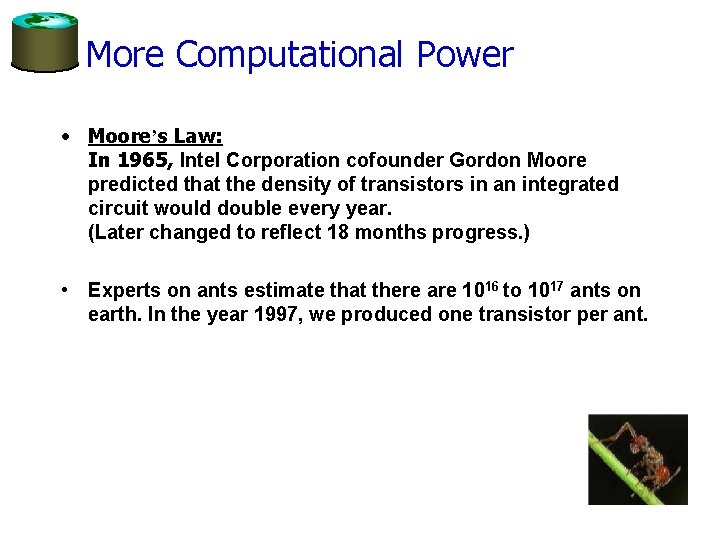
More Computational Power • Moore’s Law: In 1965, Intel Corporation cofounder Gordon Moore predicted that the density of transistors in an integrated circuit would double every year. (Later changed to reflect 18 months progress. ) • Experts on ants estimate that there are 1016 to 1017 ants on earth. In the year 1997, we produced one transistor per ant.

Much Commercial Support • Many data mining tools – http: //www. kdnuggets. com/software – http: //www. purpleinsight. com • Database systems with data mining support • Visualization tools • Data mining process support • Consultants

Why Use Data Mining Today? Competitive pressure! “The secret of success is to know something that nobody else knows. ” Aristotle Onassis • • • Competition on service, not only on price (Banks, phone companies, hotel chains, rental car companies) Personalization, CRM The real-time enterprise “Systemic listening” Security, homeland defense

The Knowledge Discovery Process Steps: l Identify business problem l Data mining l Action l Evaluation and measurement l Deployment and integration into businesses processes

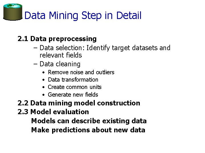
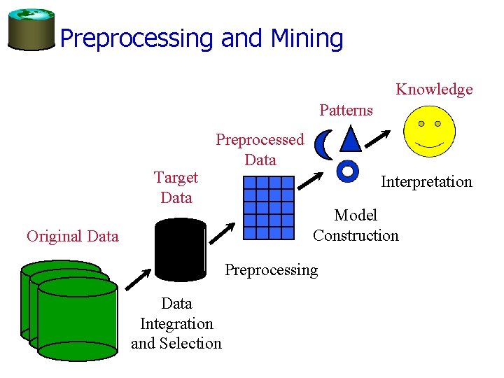
Data Mining Step in Detail 2. 1 Data preprocessing – Data selection: Identify target datasets and relevant fields – Data cleaning • • Remove noise and outliers Data transformation Create common units Generate new fields 2. 2 Data mining model construction 2. 3 Model evaluation Models can describe existing data Make predictions about new data

Preprocessing and Mining Knowledge Patterns Target Data Preprocessed Data Original Data Interpretation Model Construction Preprocessing Data Integration and Selection

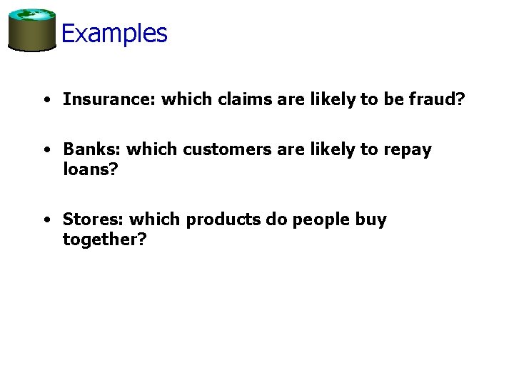
Examples • Insurance: which claims are likely to be fraud? • Banks: which customers are likely to repay loans? • Stores: which products do people buy together?

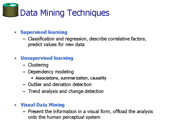
Data Mining Techniques • Supervised learning – Classification and regression, describe correlative factors, predict values for new data • Unsupervised learning – Clustering – Dependency modeling • Associations, summarization, causality – Outlier and deviation detection – Trend analysis and change detection • Visual Data Mining – Present the information in a visual form, offload the analysis onto the human perceptual system

Supervised learning • Need training data set with known outcome – e. g. here is a set of loans that were not repaid, and other loans that were repaid • Model is generated from the training set, tested on a separate test data set to determine accuracy • Model can predict outcomes on new data, – can also explain predictive factors • Examples include Decision Trees, Regression Trees, Naïve Baysian networks

Unsupervised Learning • Give data to the algorithm, it does the rest • Output might include clustered data, association rules, etc.

E. g. Agglomerative Clustering Algorithm: • Put each item in its own cluster (all singletons) • Find all pairwise distances between clusters • Merge the two closest clusters • Repeat until everything is in one cluster Observations: • Results in a hierarchical clustering • Yields a clustering for each possible number of clusters • Greedy clustering: Result is not “optimal” for any cluster size

Agglomerative Clustering Example

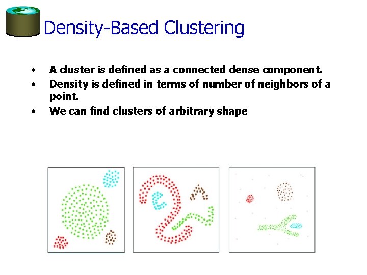
Density-Based Clustering • • • A cluster is defined as a connected dense component. Density is defined in terms of number of neighbors of a point. We can find clusters of arbitrary shape

Demo

Conclusions • Data mining very useful for understanding large data sets • Several approaches – Supervised – Unsupervised • Can describe patterns, make predictions • Many commercial packages • Many free algorithms