Relational Normalization Theory 1 Limitations of ER Designs

Relational Normalization Theory 1

Limitations of E-R Designs • Provides a set of guidelines, does not result in a unique database schema • Does not provide a way of evaluating alternative schemas • Normalization theory provides a mechanism for analyzing and refining the schema produced by an E-R design 2

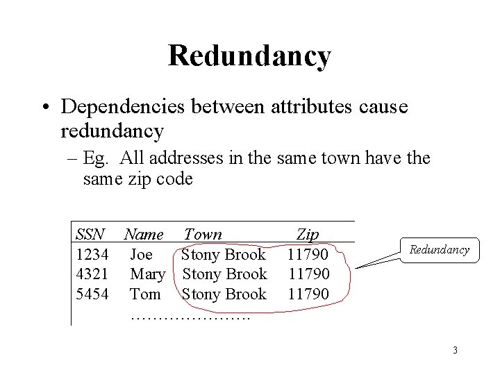
Redundancy • Dependencies between attributes cause redundancy – Eg. All addresses in the same town have the same zip code SSN Name Town 1234 Joe Stony Brook 4321 Mary Stony Brook 5454 Tom Stony Brook …………………. Zip 11790 Redundancy 3

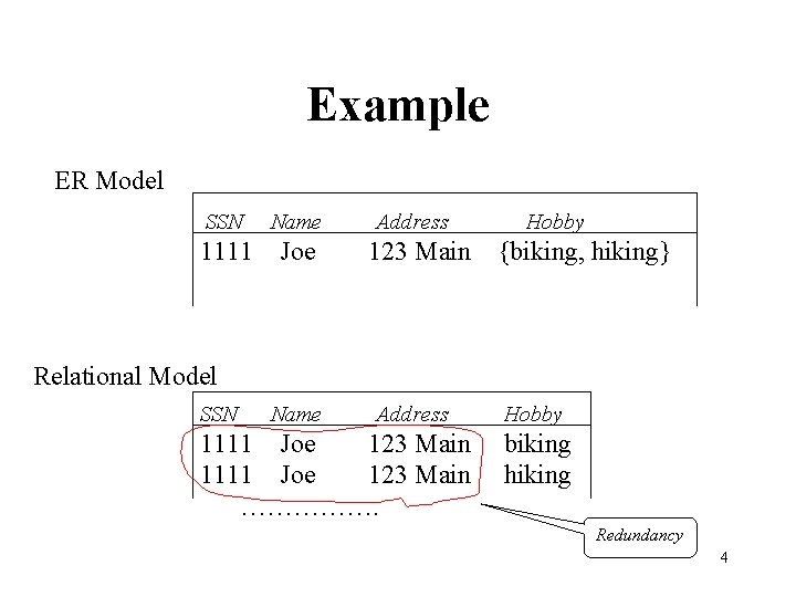
Example ER Model SSN Name 1111 Joe Address 123 Main Hobby {biking, hiking} Relational Model SSN Name Address 1111 Joe 123 Main ……………. Hobby biking hiking Redundancy 4

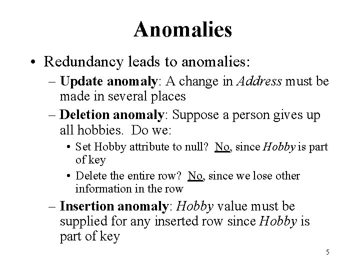
Anomalies • Redundancy leads to anomalies: – Update anomaly: A change in Address must be made in several places – Deletion anomaly: Suppose a person gives up all hobbies. Do we: • Set Hobby attribute to null? No, since Hobby is part of key • Delete the entire row? No, since we lose other information in the row – Insertion anomaly: Hobby value must be supplied for any inserted row since Hobby is part of key 5

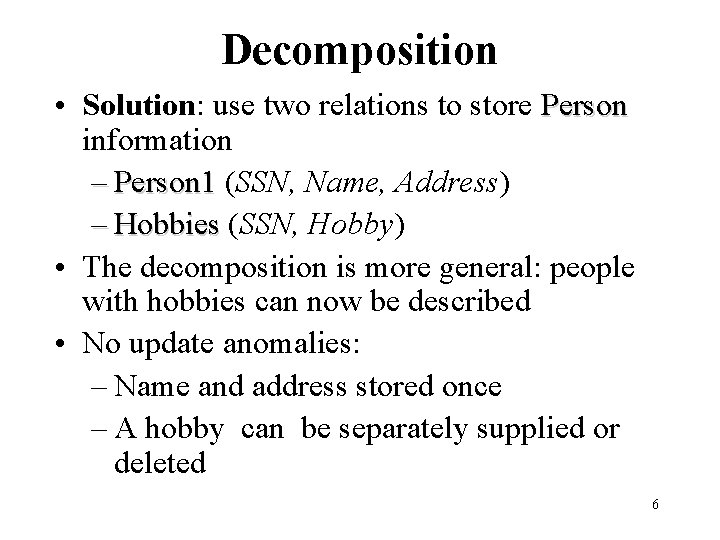
Decomposition • Solution: use two relations to store Person information – Person 1 (SSN, Name, Address) – Hobbies (SSN, Hobby) • The decomposition is more general: people with hobbies can now be described • No update anomalies: – Name and address stored once – A hobby can be separately supplied or deleted 6

Normalization Theory • Result of E-R analysis need further refinement • Appropriate decomposition can solve problems • The underlying theory is referred to as normalization theory and is based on functional dependencies (and other kinds, like multi-valued dependencies) dependencies 7

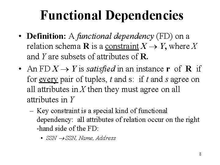
Functional Dependencies • Definition: A functional dependency (FD) on a relation schema R is a constraint X Y, where X and Y are subsets of attributes of R. • An FD X Y is satisfied in an instance r of R if for every pair of tuples, t and s: if t and s agree on all attributes in X then they must agree on all attributes in Y – Key constraint is a special kind of functional dependency: all attributes of relation occur on the right -hand side of the FD: • SSN, Name, Address 8

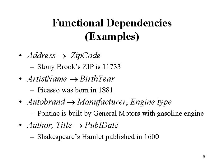
Functional Dependencies (Examples) • Address Zip. Code – Stony Brook’s ZIP is 11733 • Artist. Name Birth. Year – Picasso was born in 1881 • Autobrand Manufacturer, Engine type – Pontiac is built by General Motors with gasoline engine • Author, Title Publ. Date – Shakespeare’s Hamlet published in 1600 9

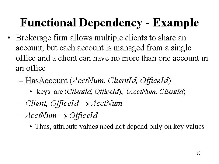
Functional Dependency - Example • Brokerage firm allows multiple clients to share an account, but each account is managed from a single office and a client can have no more than one account in an office – Has. Account (Acct. Num, Client. Id, Office. Id) • keys are (Client. Id, Office. Id), (Acct. Num, Client. Id) – Client, Office. Id Acct. Num – Acct. Num Office. Id • Thus, attribute values need not depend only on key values 10

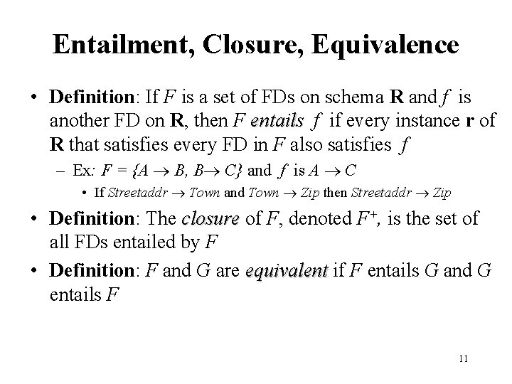
Entailment, Closure, Equivalence • Definition: If F is a set of FDs on schema R and f is another FD on R, then F entails f if every instance r of R that satisfies every FD in F also satisfies f – Ex: F = {A B, B C} and f is A C • If Streetaddr Town and Town Zip then Streetaddr Zip • Definition: The closure of F, denoted F+, is the set of all FDs entailed by F • Definition: F and G are equivalent if F entails G and G entails F 11

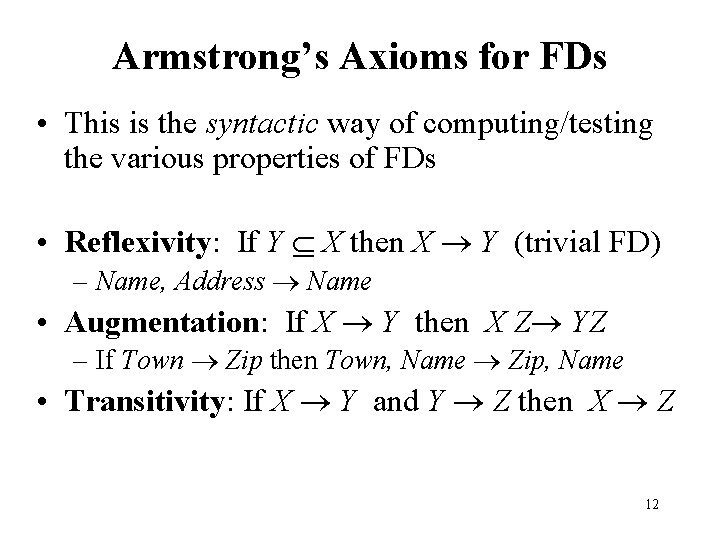
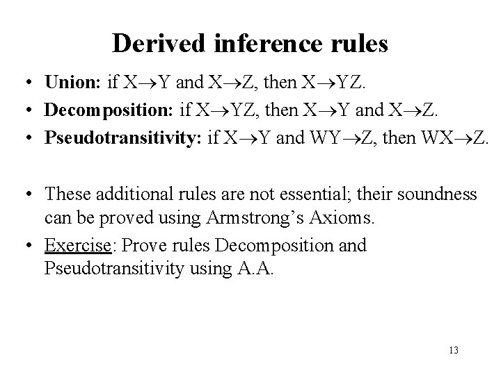
Armstrong’s Axioms for FDs • This is the syntactic way of computing/testing the various properties of FDs • Reflexivity: If Y X then X Y (trivial FD) – Name, Address Name • Augmentation: If X Y then X Z YZ – If Town Zip then Town, Name Zip, Name • Transitivity: If X Y and Y Z then X Z 12

Derived inference rules • Union: if X Y and X Z, then X YZ. • Decomposition: if X YZ, then X Y and X Z. • Pseudotransitivity: if X Y and WY Z, then WX Z. • These additional rules are not essential; their soundness can be proved using Armstrong’s Axioms. • Exercise: Prove rules Decomposition and Pseudotransitivity using A. A. 13

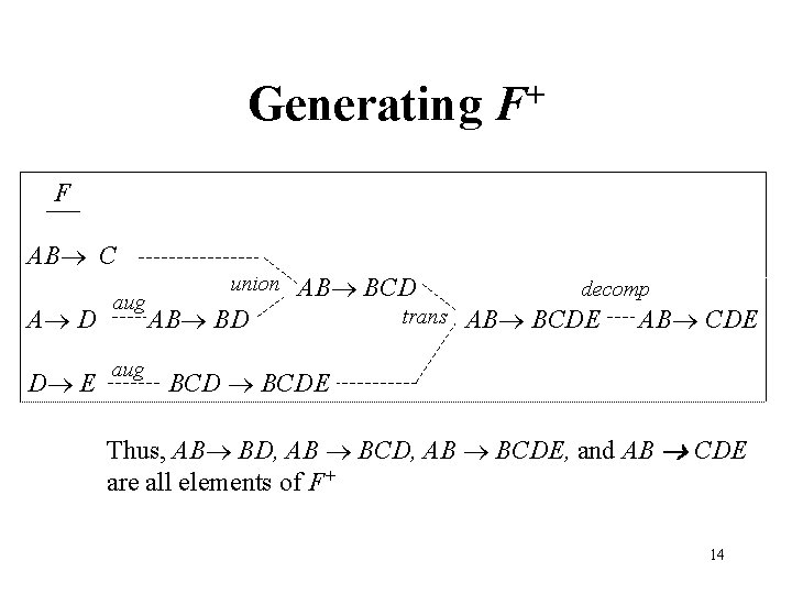
Generating + F F AB C A D D E aug union AB BCD AB BD trans decomp AB BCDE AB CDE BCDE Thus, AB BD, AB BCDE, and AB CDE are all elements of F+ 14

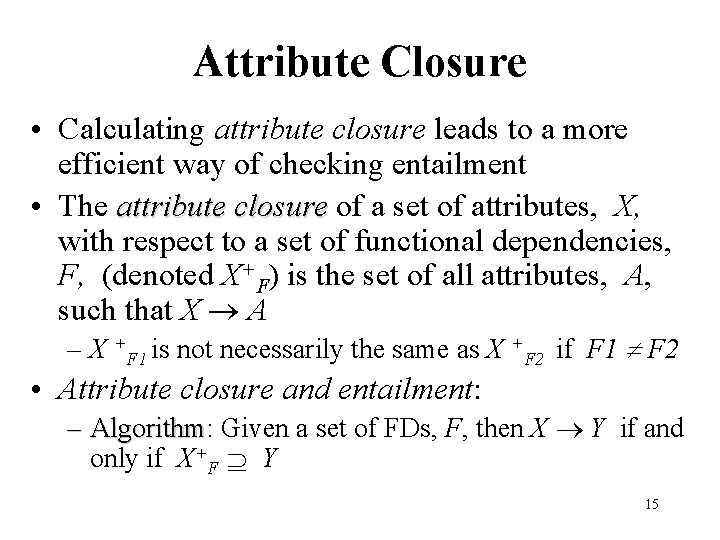
Attribute Closure • Calculating attribute closure leads to a more efficient way of checking entailment • The attribute closure of a set of attributes, X, with respect to a set of functional dependencies, F, (denoted X+F) is the set of all attributes, A, such that X A – X +F 1 is not necessarily the same as X +F 2 if F 1 F 2 • Attribute closure and entailment: – Algorithm: Algorithm Given a set of FDs, F, then X Y if and only if X+F Y 15

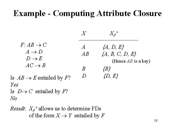
Example - Computing Attribute Closure X F: AB C A D D E AC B Is AB E entailed by F? Yes Is D C entailed by F? No A AB X F+ {A, D, E} {A, B, C, D, E} (Hence AB is a key) B D {B} {D, E} Result: XF+ allows us to determine FDs of the form X Y entailed by F 16

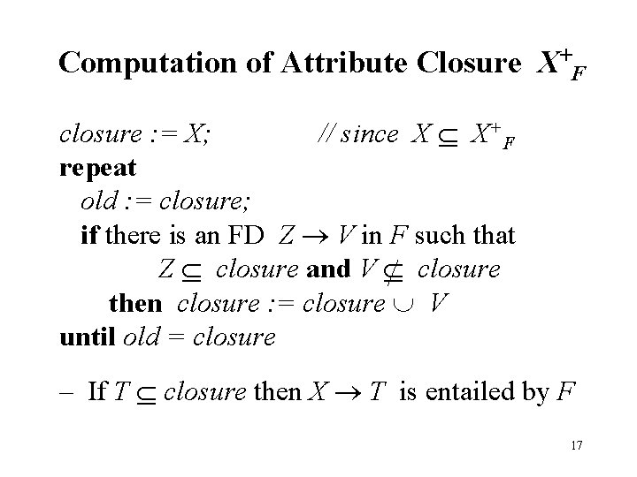
Computation of Attribute Closure X+F closure : = X; // since X X+F repeat old : = closure; if there is an FD Z V in F such that Z closure and V closure then closure : = closure V until old = closure – If T closure then X T is entailed by F 17

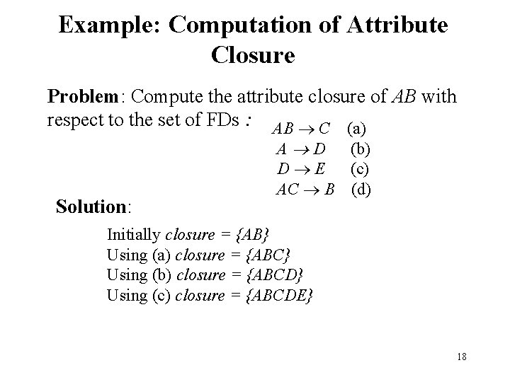
Example: Computation of Attribute Closure Problem: Compute the attribute closure of AB with respect to the set of FDs : AB C (a) Solution: A D (b) D E (c) AC B (d) Initially closure = {AB} Using (a) closure = {ABC} Using (b) closure = {ABCD} Using (c) closure = {ABCDE} 18

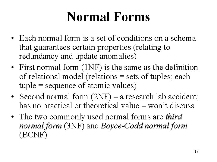
Normal Forms • Each normal form is a set of conditions on a schema that guarantees certain properties (relating to redundancy and update anomalies) • First normal form (1 NF) is the same as the definition of relational model (relations = sets of tuples; each tuple = sequence of atomic values) • Second normal form (2 NF) – a research lab accident; has no practical or theoretical value – won’t discuss • The two commonly used normal forms are third normal form (3 NF) and Boyce-Codd normal form (BCNF) 19

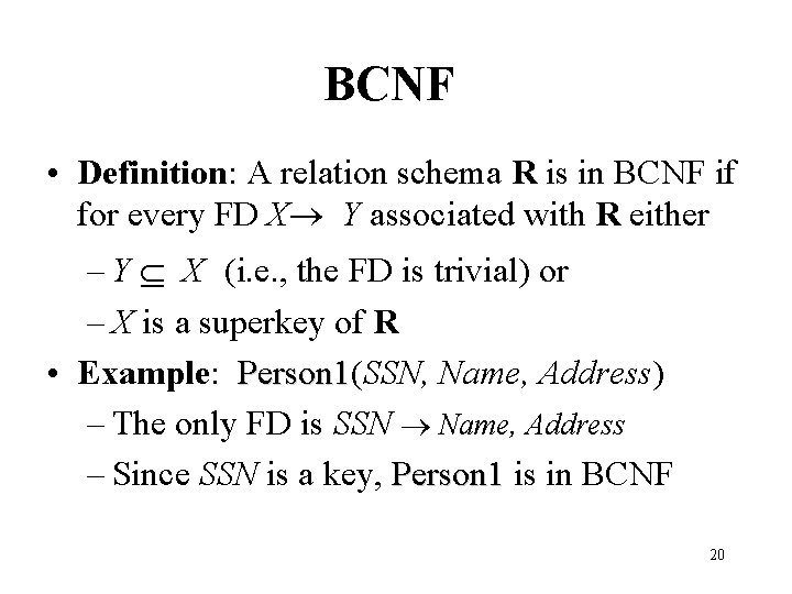
BCNF • Definition: A relation schema R is in BCNF if for every FD X Y associated with R either – Y X (i. e. , the FD is trivial) or – X is a superkey of R • Example: Person 1(SSN, Name, Address) Person 1 – The only FD is SSN Name, Address – Since SSN is a key, Person 1 is in BCNF 20

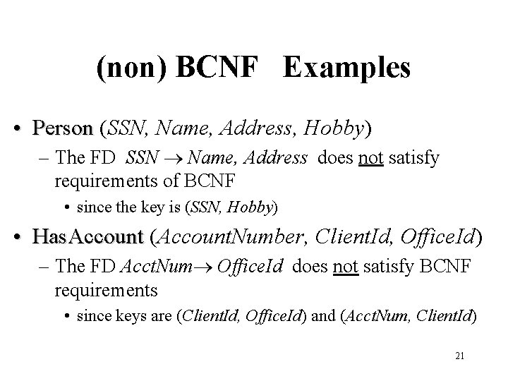
(non) BCNF Examples • Person (SSN, Name, Address, Hobby) – The FD SSN Name, Address does not satisfy requirements of BCNF • since the key is (SSN, Hobby) • Has. Account (Account. Number, Client. Id, Office. Id) – The FD Acct. Num Office. Id does not satisfy BCNF requirements • since keys are (Client. Id, Office. Id) and (Acct. Num, Client. Id) 21

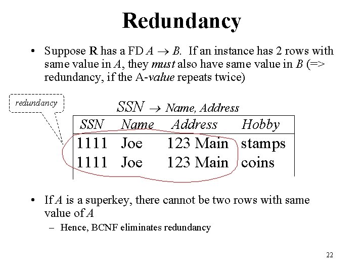
Redundancy • Suppose R has a FD A B. If an instance has 2 rows with same value in A, they must also have same value in B (=> redundancy, if the A-value repeats twice) SSN redundancy SSN Name 1111 Joe Name, Address Hobby 123 Main stamps 123 Main coins • If A is a superkey, there cannot be two rows with same value of A – Hence, BCNF eliminates redundancy 22

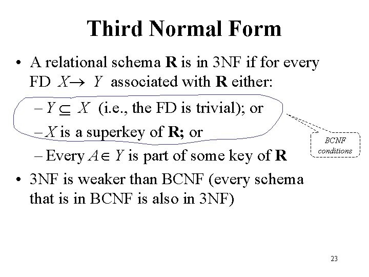
Third Normal Form • A relational schema R is in 3 NF if for every FD X Y associated with R either: – Y X (i. e. , the FD is trivial); or – X is a superkey of R; or – Every A Y is part of some key of R • 3 NF is weaker than BCNF (every schema that is in BCNF is also in 3 NF) BCNF conditions 23

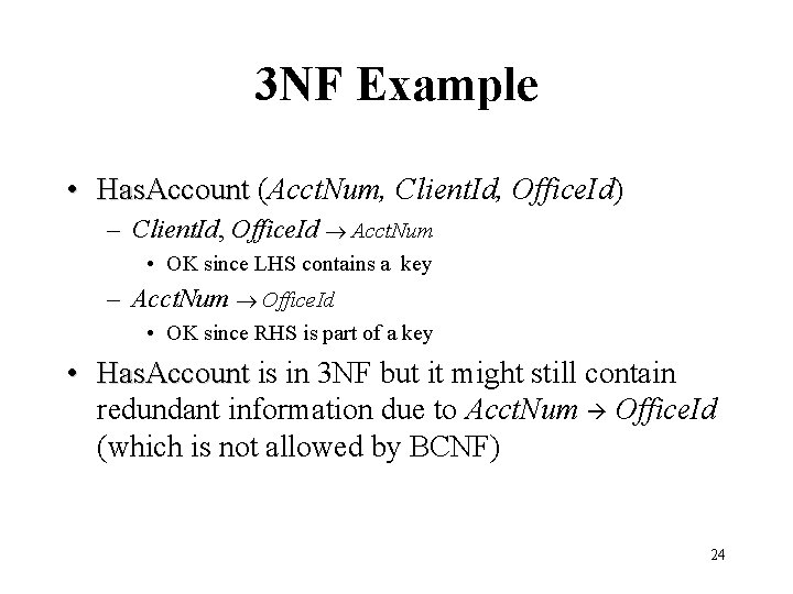
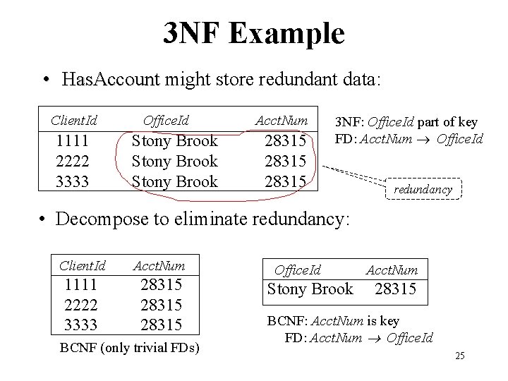
3 NF Example • Has. Account (Acct. Num, Client. Id, Office. Id) – Client. Id, Office. Id Acct. Num • OK since LHS contains a key – Acct. Num Office. Id • OK since RHS is part of a key • Has. Account is in 3 NF but it might still contain redundant information due to Acct. Num Office. Id (which is not allowed by BCNF) 24

3 NF Example • Has. Account might store redundant data: Client. Id 1111 2222 3333 Office. Id Stony Brook Acct. Num 28315 3 NF: Office. Id part of key FD: Acct. Num Office. Id redundancy • Decompose to eliminate redundancy: Client. Id Acct. Num 1111 2222 3333 28315 BCNF (only trivial FDs) Office. Id Stony Brook Acct. Num 28315 BCNF: Acct. Num is key FD: Acct. Num Office. Id 25

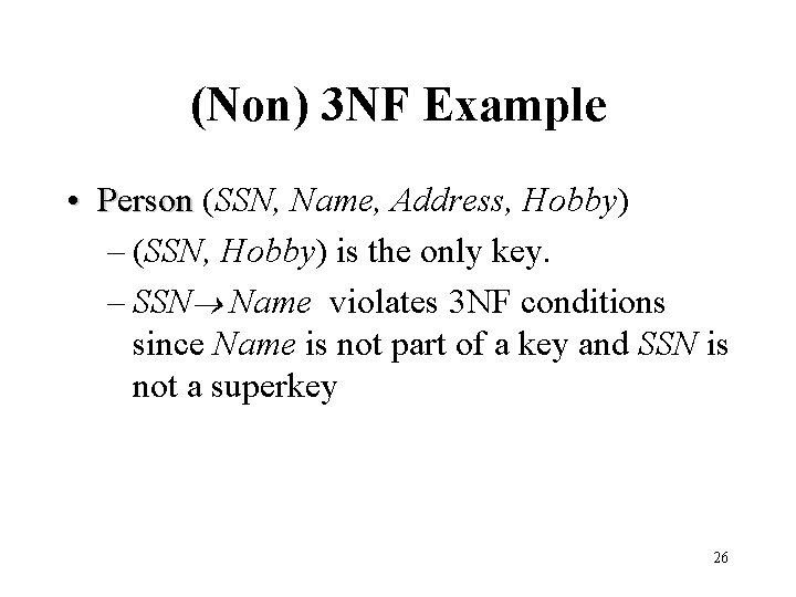
(Non) 3 NF Example • Person (SSN, Name, Address, Hobby) – (SSN, Hobby) is the only key. – SSN Name violates 3 NF conditions since Name is not part of a key and SSN is not a superkey 26

Decompositions • Goal: Eliminate redundancy by decomposing a relation into several relations in a higher normal form • Decomposition must be lossless: lossless it must be possible to reconstruct the original relation from the relations in the decomposition • We will see why 27

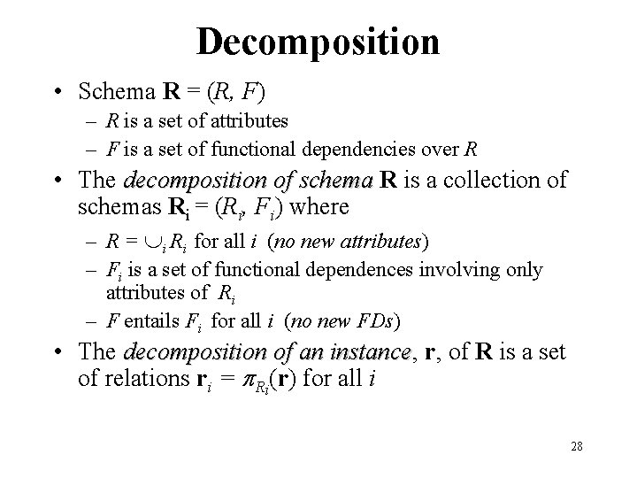
Decomposition • Schema R = (R, F) – R is a set of attributes – F is a set of functional dependencies over R • The decomposition of schema R is a collection of schemas Ri = (Ri, Fi) where – R = i Ri for all i (no new attributes) – Fi is a set of functional dependences involving only attributes of Ri – F entails Fi for all i (no new FDs) • The decomposition of an instance, instance r, of R is a set of relations ri = Ri(r) for all i 28

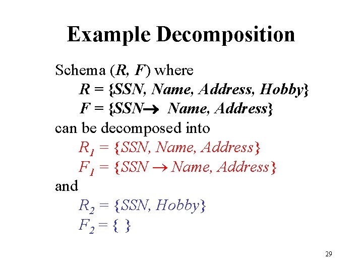
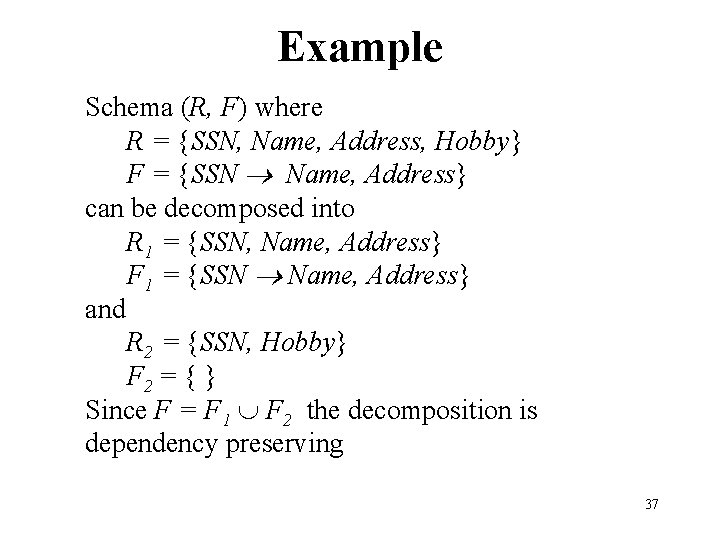
Example Decomposition Schema (R, F) where R = {SSN, Name, Address, Hobby} F = {SSN Name, Address} can be decomposed into R 1 = {SSN, Name, Address} F 1 = {SSN Name, Address} and R 2 = {SSN, Hobby} F 2 = { } 29

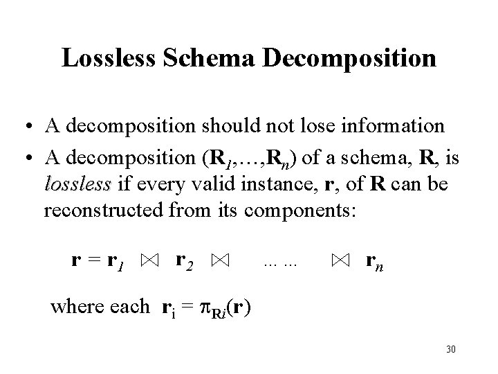
Lossless Schema Decomposition • A decomposition should not lose information • A decomposition (R 1, …, Rn) of a schema, R, is lossless if every valid instance, r, of R can be reconstructed from its components: r = r 1 r 2 …… rn where each ri = Ri(r) 30

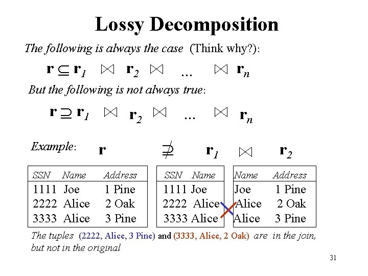
Lossy Decomposition The following is always the case (Think why? ): r r 1 r 2 rn . . . But the following is not always true: r r 1 Example: SSN Name 1111 Joe 2222 Alice 3333 Alice r 2 r . . . rn r 1 Address SSN Name 1 Pine 2 Oak 3 Pine 1111 Joe 2222 Alice 3333 Alice r 2 Name Address Joe Alice 1 Pine 2 Oak 3 Pine The tuples (2222, Alice, 3 Pine) and (3333, Alice, 2 Oak) are in the join, but not in the original 31

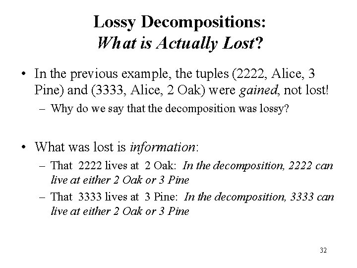
Lossy Decompositions: What is Actually Lost? • In the previous example, the tuples (2222, Alice, 3 Pine) and (3333, Alice, 2 Oak) were gained, not lost! – Why do we say that the decomposition was lossy? • What was lost is information: – That 2222 lives at 2 Oak: In the decomposition, 2222 can live at either 2 Oak or 3 Pine – That 3333 lives at 3 Pine: In the decomposition, 3333 can live at either 2 Oak or 3 Pine 32

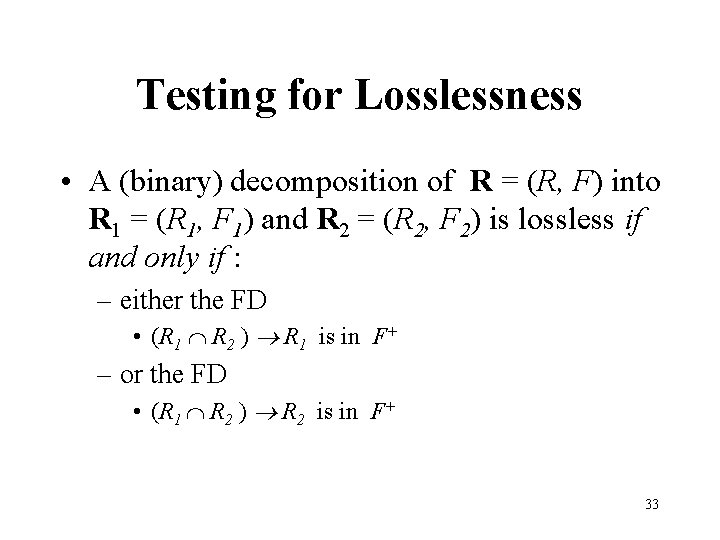
Testing for Losslessness • A (binary) decomposition of R = (R, F) into R 1 = (R 1, F 1) and R 2 = (R 2, F 2) is lossless if and only if : – either the FD • (R 1 R 2 ) R 1 is in F+ – or the FD • (R 1 R 2 ) R 2 is in F+ 33

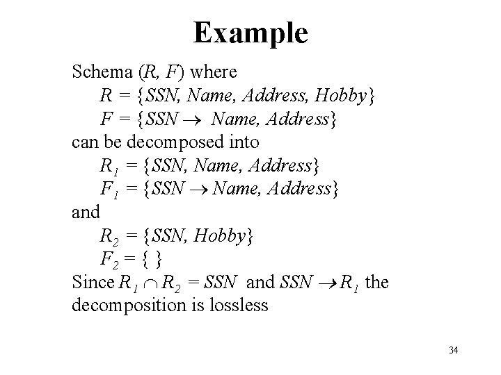
Example Schema (R, F) where R = {SSN, Name, Address, Hobby} F = {SSN Name, Address} can be decomposed into R 1 = {SSN, Name, Address} F 1 = {SSN Name, Address} and R 2 = {SSN, Hobby} F 2 = { } Since R 1 R 2 = SSN and SSN R 1 the decomposition is lossless 34

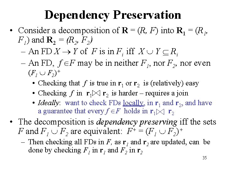
Dependency Preservation • Consider a decomposition of R = (R, F) into R 1 = (R 1, F 1) and R 2 = (R 2, F 2) – An FD X Y of F is in Fi iff X Y Ri – An FD, f F may be in neither F 1, nor F 2, nor even (F 1 F 2)+ • Checking that f is true in r 1 or r 2 is (relatively) easy • Checking f in r 1 r 2 is harder – requires a join • Ideally: want to check FDs locally, in r 1 and r 2, and have a guarantee that every f F holds in r 1 r 2 • The decomposition is dependency preserving iff the sets F and F 1 F 2 are equivalent: F+ = (F 1 F 2)+ – Then checking all FDs in F, as r 1 and r 2 are updated, can be done by checking F 1 in r 1 and F 2 in r 2 35

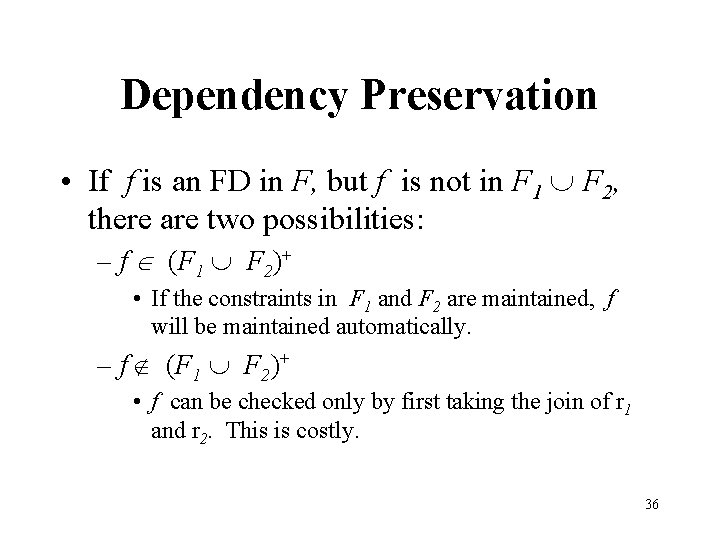
Dependency Preservation • If f is an FD in F, but f is not in F 1 F 2, there are two possibilities: – f (F 1 F 2)+ • If the constraints in F 1 and F 2 are maintained, f will be maintained automatically. – f (F 1 F 2)+ • f can be checked only by first taking the join of r 1 and r 2. This is costly. 36

Example Schema (R, F) where R = {SSN, Name, Address, Hobby} F = {SSN Name, Address} can be decomposed into R 1 = {SSN, Name, Address} F 1 = {SSN Name, Address} and R 2 = {SSN, Hobby} F 2 = { } Since F = F 1 F 2 the decomposition is dependency preserving 37

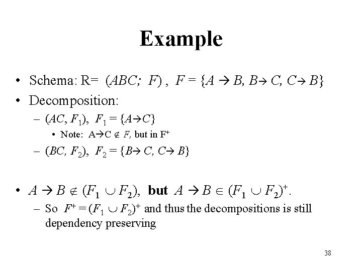
Example • Schema: R= (ABC; F) , F = {A B, B C, C B} • Decomposition: – (AC, F 1), F 1 = {A C} • Note: A C F, but in F+ – (BC, F 2), F 2 = {B C, C B} • A B (F 1 F 2), but A B (F 1 F 2)+. – So F+ = (F 1 F 2)+ and thus the decompositions is still dependency preserving 38

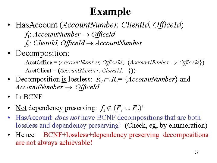
Example • Has. Account (Account. Number, Client. Id, Office. Id) f 1: Account. Number Office. Id f 2: Client. Id, Office. Id Account. Number • Decomposition: Acct. Office = (Account. Number, Office. Id; {Account. Number Office. Id}) Acct. Client = (Account. Number, Client. Id; {}) • Decomposition is lossless: R 1 R 2= {Account. Number} and Account. Number Office. Id • In BCNF • Not dependency preserving: f 2 (F 1 F 2)+ • Has. Account does not have BCNF decompositions that are both lossless and dependency preserving! (Check, eg, by enumeration) • Hence: BCNF+lossless+dependency preserving decompositions are not always achievable! 39

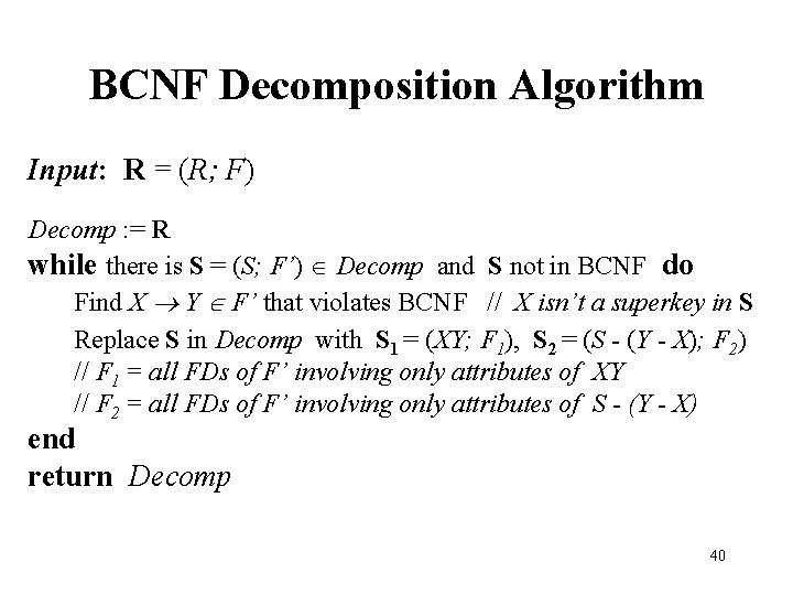
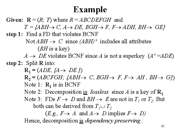
BCNF Decomposition Algorithm Input: R = (R; F) Decomp : = R while there is S = (S; F’) Decomp and S not in BCNF do Find X Y F’ that violates BCNF // X isn’t a superkey in S Replace S in Decomp with S 1 = (XY; F 1), S 2 = (S - (Y - X); F 2) // F 1 = all FDs of F’ involving only attributes of XY // F 2 = all FDs of F’ involving only attributes of S - (Y - X) end return Decomp 40

Example Given: R = (R; T) where R = ABCDEFGH and T = {ABH C, A DE, BGH F, F ADH, BH GE} step 1: Find a FD that violates BCNF Not ABH C since (ABH)+ includes all attributes (BH is a key) A DE violates BCNF since A is not a superkey (A+ =ADE) step 2: Split R into: R 1 = (ADE, {A DE }) R 2 = (ABCFGH; {ABH C, BGH F, F AH , BH G}) Note 1: R 1 is in BCNF Note 2: Decomposition is lossless since A is a key of R 1. Note 3: FDs F D and BH E are not in T 1 or T 2. But both can be derived from T 1 T 2 (E. g. , F A and A D implies F D) Hence, decomposition is dependency preserving. 41

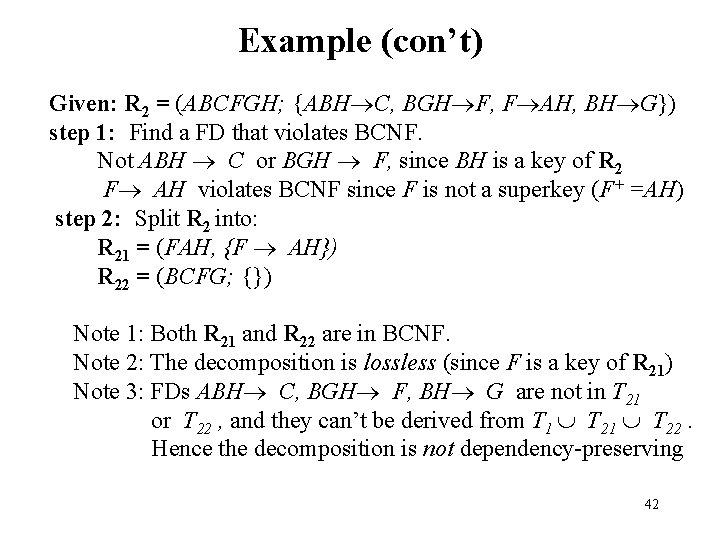
Example (con’t) Given: R 2 = (ABCFGH; {ABH C, BGH F, F AH, BH G}) step 1: Find a FD that violates BCNF. Not ABH C or BGH F, since BH is a key of R 2 F AH violates BCNF since F is not a superkey (F+ =AH) step 2: Split R 2 into: R 21 = (FAH, {F AH}) R 22 = (BCFG; {}) Note 1: Both R 21 and R 22 are in BCNF. Note 2: The decomposition is lossless (since F is a key of R 21) Note 3: FDs ABH C, BGH F, BH G are not in T 21 or T 22 , and they can’t be derived from T 1 T 22. Hence the decomposition is not dependency-preserving 42

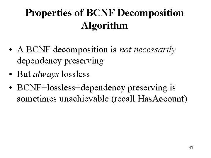
Properties of BCNF Decomposition Algorithm • A BCNF decomposition is not necessarily dependency preserving • But always lossless • BCNF+lossless+dependency preserving is sometimes unachievable (recall Has. Account) Has. Account 43

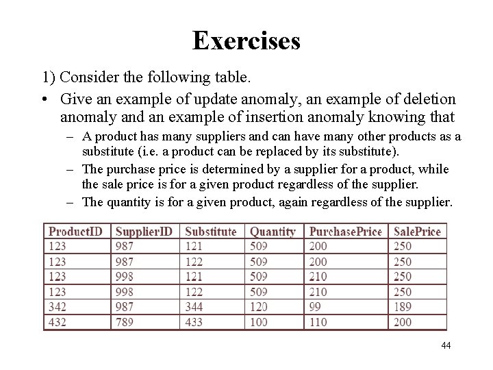
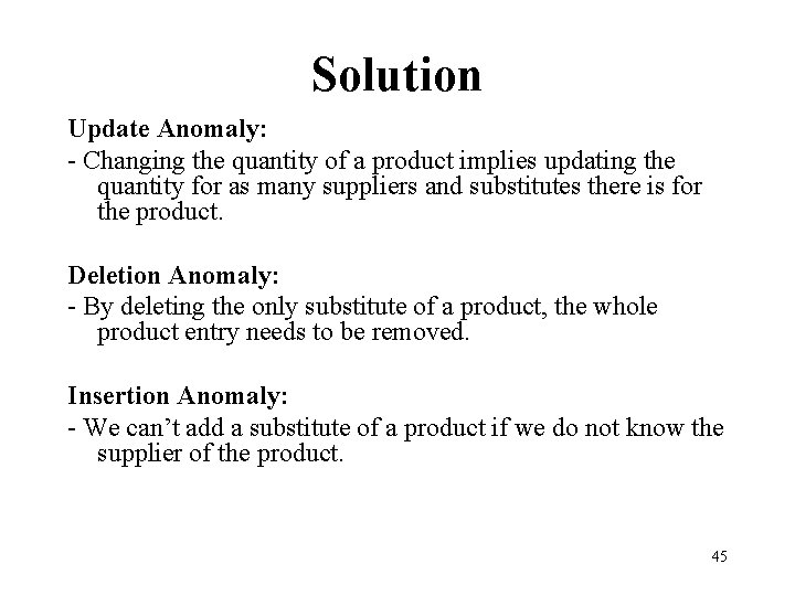
Exercises 1) Consider the following table. • Give an example of update anomaly, an example of deletion anomaly and an example of insertion anomaly knowing that – A product has many suppliers and can have many other products as a substitute (i. e. a product can be replaced by its substitute). – The purchase price is determined by a supplier for a product, while the sale price is for a given product regardless of the supplier. – The quantity is for a given product, again regardless of the supplier. 44

Solution Update Anomaly: - Changing the quantity of a product implies updating the quantity for as many suppliers and substitutes there is for the product. Deletion Anomaly: - By deleting the only substitute of a product, the whole product entry needs to be removed. Insertion Anomaly: - We can’t add a substitute of a product if we do not know the supplier of the product. 45

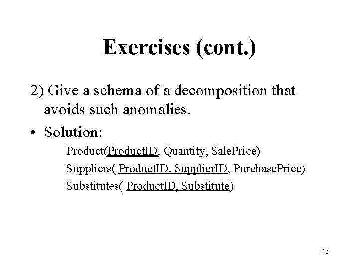
Exercises (cont. ) 2) Give a schema of a decomposition that avoids such anomalies. • Solution: Product(Product. ID, Quantity, Sale. Price) Suppliers( Product. ID, Supplier. ID, Purchase. Price) Substitutes( Product. ID, Substitute) 46

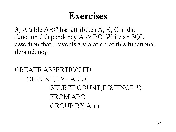
Exercises 3) A table ABC has attributes A, B, C and a functional dependency A -> BC. Write an SQL assertion that prevents a violation of this functional dependency. CREATE ASSERTION FD CHECK (1 >= ALL ( SELECT COUNT(DISTINCT *) FROM ABC GROUP BY A ) ) 47

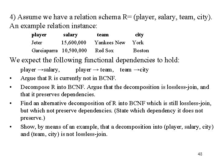
4) Assume we have a relation schema R= (player, salary, team, city). An example relation instance: player salary Jeter 15, 600, 000 Garciaparra 10, 500, 000 team Yankees New Red Sox city York Boston We expect the following functional dependencies to hold: • • player →salary, player → team, team →city Argue that R is currently not in BCNF. Decompose R into BCNF. Argue that the decomposition is lossless-join, and that it preserves dependencies. Find an alternative decomposition of R into BCNF which is still lossless-join, but which not preserve dependencies. (State which dependency it does not preserve. ) Show, by means of an example, that a decomposition into (player, salary, city) and (team, city) is not lossless-join. 48