Random Sets Approach and its Applications Vladimir Nikulin

Random Sets Approach and its Applications Vladimir Nikulin, Suncorp, Australia • Introduction: input data, objectives and main assumptions. • • Basic iterative feature selection, and modifications. • Tests for independence & trimmings (similar to HITON algorithm). • Experimental results with some comments. • Concluding remarks. Random sets approach. 1

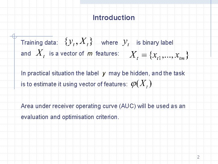
Introduction Training data: and where is binary label is a vector of m features: In practical situation the label y may be hidden, and the task is to estimate it using vector of features: Area under receiver operating curve (AUC) will be used as an evaluation and optimisation criterion. 2

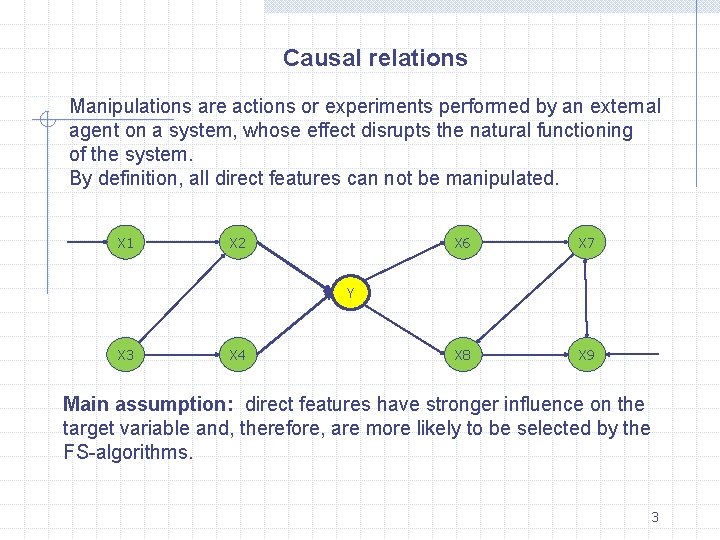
Causal relations Manipulations are actions or experiments performed by an external agent on a system, whose effect disrupts the natural functioning of the system. By definition, all direct features can not be manipulated. X 1 X 2 X 6 X 7 X 8 X 9 Y X 3 X 4 Main assumption: direct features have stronger influence on the target variable and, therefore, are more likely to be selected by the FS-algorithms. 3

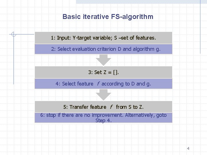
Basic iterative FS-algorithm 1: Input: Y-target variable; S –set of features. 2: Select evaluation criterion D and algorithm g. 3: Set Z = []. 4: Select feature f according to D and g. 5: Transfer feature f from S to Z. 6: stop if there are no improvement. Alternatively, goto Step 4. 4

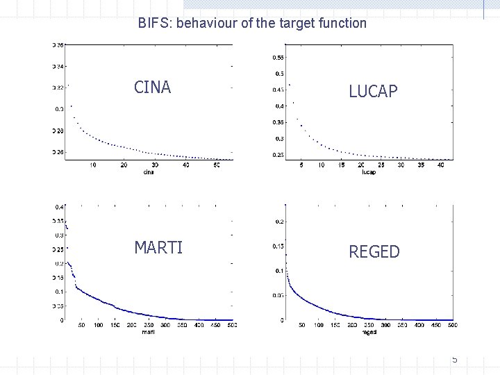
BIFS: behaviour of the target function CINA LUCAP MARTI REGED 5

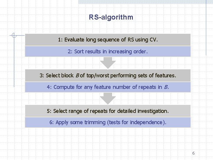
RS-algorithm 1: Evaluate long sequence of RS using CV. 2: Sort results in increasing order. 3: Select block B of top/worst performing sets of features. 4: Compute for any feature number of repeats in B. 5: Select range of repeats for detailed investigation. 6: Apply some trimming (tests for independence). 6

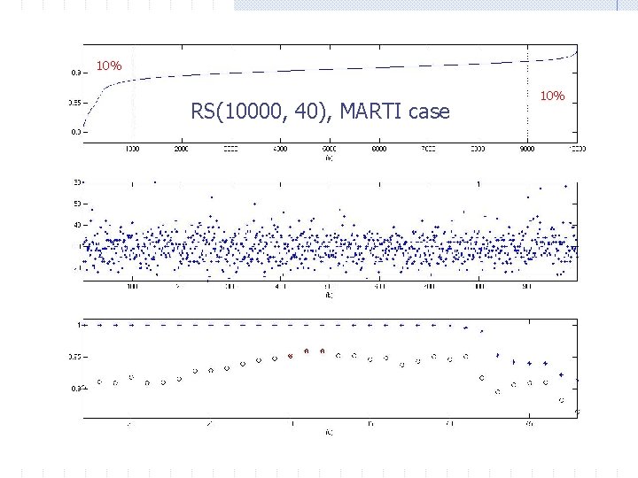
10% RS(10000, 40), MARTI case 10% 7

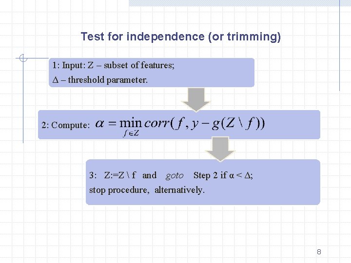
Test for independence (or trimming) 1: Input: Z – subset of features; Δ – threshold parameter. 2: Compute: 3: Z: =Z f and goto Step 2 if α < Δ; stop procedure, alternatively. 8

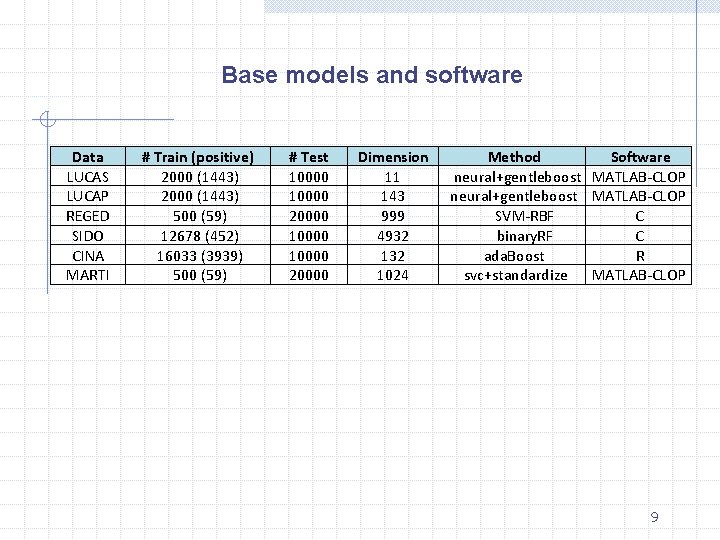
Base models and software Data LUCAS LUCAP REGED SIDO CINA MARTI # Train (positive) 2000 (1443) 500 (59) 12678 (452) 16033 (3939) 500 (59) # Test 10000 20000 Dimension 11 143 999 4932 1024 Method Software neural+gentleboost MATLAB-CLOP SVM-RBF C binary. RF C ada. Boost R svc+standardize MATLAB-CLOP 9

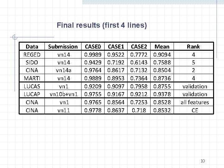
Final results (first 4 lines) Data REGED SIDO CINA MARTI LUCAS LUCAP CINA Submission vn 14 a vn 14 vn 10 b+vn 11 CASE 0 0. 9989 0. 9429 0. 9764 0. 9889 0. 9209 0. 9755 0. 9765 0. 9778 CASE 1 0. 9522 0. 7192 0. 8617 0. 8953 0. 9097 0. 9167 0. 8564 0. 8637 CASE 2 0. 7772 0. 6143 0. 7132 0. 7364 0. 7958 0. 9212 0. 7253 0. 718 Mean 0. 9094 0. 7588 0. 8504 0. 8736 0. 8755 0. 9378 0. 8528 0. 8532 Rank 4 5 2 4 validation all features CE 10

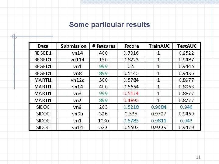
Some particular results Data REGED 1 MARTI 1 SIDO 0 Submission vn 14 vn 11 d vn 1 vn 8 vn 12 c vn 14 vn 3 vn 7 vn 9 a vn 14 # features 400 150 999 899 500 400 999 899 203 326 1030 527 Fscore 0. 7316 0. 8223 0. 5145 0. 5784 0. 5554 0. 5124 0. 4895 0. 5218 0. 536 0. 5785 0. 5502 Train. AUC 1 1 1 1 0. 9684 0. 9727 0. 9811 0. 9779 Test. AUC 0. 9522 0. 9487 0. 9445 0. 9436 0. 8977 0. 8953 0. 8872 0. 8722 0. 946 0. 9459 0. 943 0. 9429 11

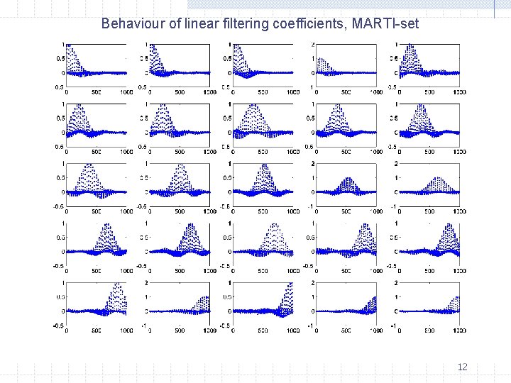
Behaviour of linear filtering coefficients, MARTI-set 12

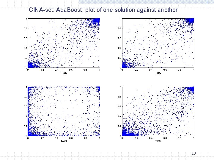
CINA-set: Ada. Boost, plot of one solution against another 13

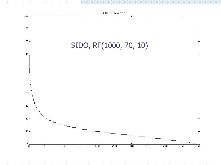
SIDO, RF(1000, 70, 10) 14

Some comments In practical applications we are dealing not with pure probability distributions, but with mixtures of distributions, which reflect changing in time trends and patterns. Accordingly, it appears to be more natural to form training set as an unlabeled mixture of subsets derived from different (manipulated) distributions, for example, REGED 1, REGED 2, . . , REGED 9. As a distribution for the test set we can select any “pure” distribution. Proper validation is particularly important in the case when training and test sets have different distributions. Respectively, it will be good to apply traditional strategy: split randomly available test-set into 2 parts 50/50 where one part will be used for validation, second part for testing. 15

Concluding remarks Random sets approach has heuristic nature and has been inspired by the growing speed of computations. It is general method, and there are many ways for further developments. Performance of the model depends on the particular data. Definitely, we can not expect that one method will produce good solutions for all problems. Probably, it was necessary to apply more aggressive FS-strategy in the case of Causal Discovery competition. Our results against all unmanipulated and all validation sets are in line with top results. 16