Queuing Models J Mercy Arokia Rani Assistant Professor

Queuing Models J. Mercy Arokia Rani Assistant Professor Department of Mathematics St. Joseph’s College(autonomous) Trichy – 620 002

Queuing or Waiting Line Analysis • Queues (waiting lines) affect people everyday • A primary goal is finding the best level of service • Analytical modeling (using formulas) can be used for many queues • For more complex situations, computer simulation is needed

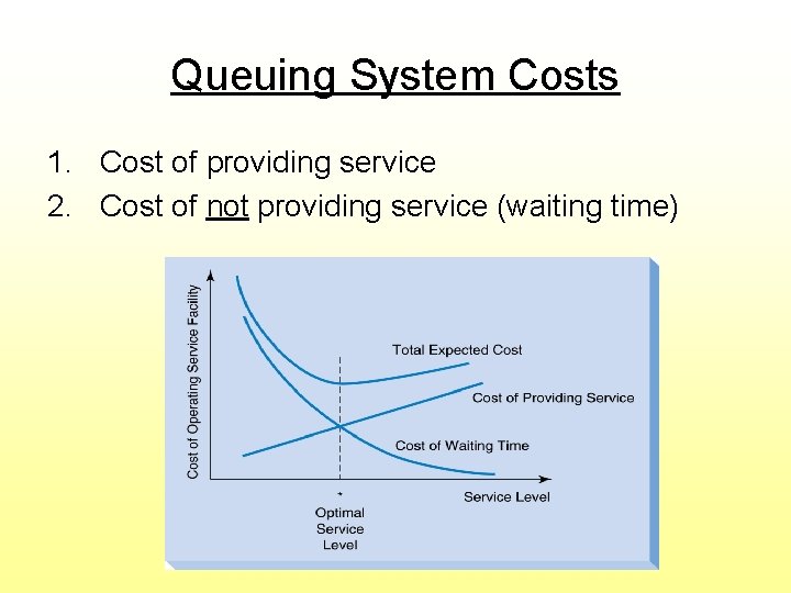
Queuing System Costs 1. Cost of providing service 2. Cost of not providing service (waiting time)

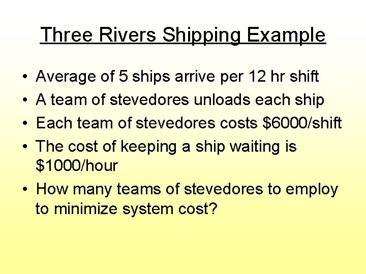
Three Rivers Shipping Example • • Average of 5 ships arrive per 12 hr shift A team of stevedores unloads each ship Each team of stevedores costs $6000/shift The cost of keeping a ship waiting is $1000/hour • How many teams of stevedores to employ to minimize system cost?

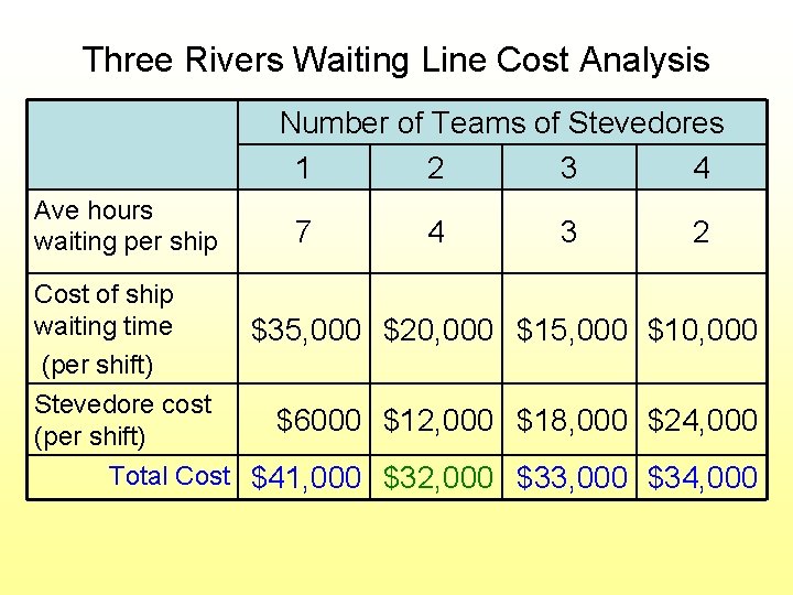
Three Rivers Waiting Line Cost Analysis Number of Teams of Stevedores 1 2 3 4 Ave hours waiting per ship Cost of ship waiting time (per shift) Stevedore cost (per shift) 7 4 3 2 $35, 000 $20, 000 $15, 000 $10, 000 $6000 $12, 000 $18, 000 $24, 000 Total Cost $41, 000 $32, 000 $33, 000 $34, 000

Characteristics of a Queuing System The queuing system is determined by: • Arrival characteristics • Queue characteristics • Service facility characteristics

Arrival Characteristics • Size of the arrival population – either infinite or limited • Arrival distribution: – Either fixed or random – Either measured by time between consecutive arrivals, or arrival rate – The Poisson distribution is often used for random arrivals

Poisson Distribution • Average arrival rate is known • Average arrival rate is constant for some number of time periods • Number of arrivals in each time period is independent • As the time interval approaches 0, the average number of arrivals approaches 0

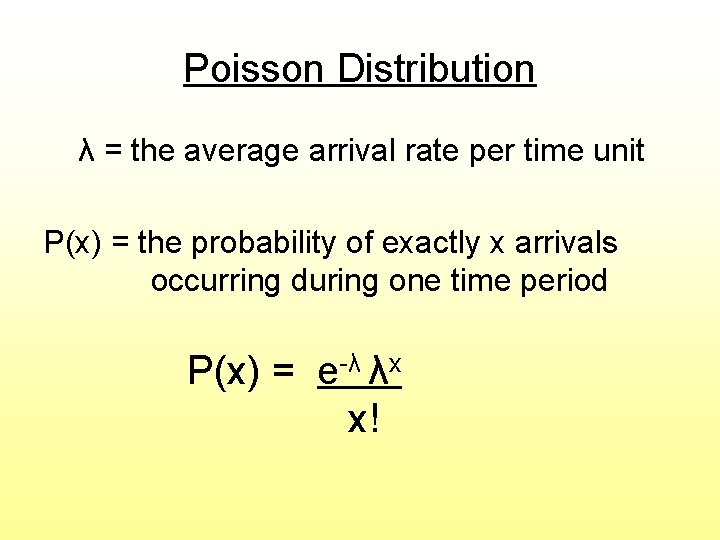
Poisson Distribution λ = the average arrival rate per time unit P(x) = the probability of exactly x arrivals occurring during one time period P(x) = e-λ λx x!

Behavior of Arrivals • Most queuing formulas assume that all arrivals stay until service is completed • Balking refers to customers who do not join the queue • Reneging refers to customers who join the queue but give up and leave before completing service

Queue Characteristics • Queue length (max possible queue length) – either limited or unlimited • Service discipline – usually FIFO (First In First Out)

Service Facility Characteristics 1. Configuration of service facility • Number of servers (or channels) • Number of phases (or service stops) 2. Service distribution • The time it takes to serve 1 arrival • Can be fixed or random • Exponential distribution is often used

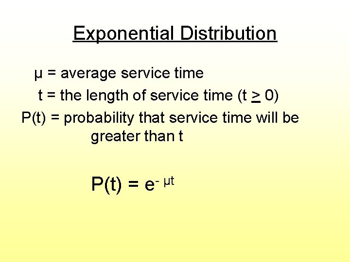
Exponential Distribution μ = average service time t = the length of service time (t > 0) P(t) = probability that service time will be greater than t P(t) = e- μt

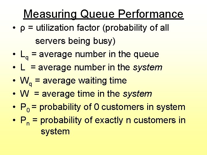
Measuring Queue Performance • ρ = utilization factor (probability of all servers being busy) • Lq = average number in the queue • L = average number in the system • Wq = average waiting time • W = average time in the system • P 0 = probability of 0 customers in system • Pn = probability of exactly n customers in system

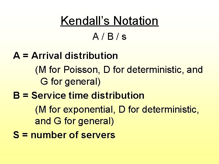
Kendall’s Notation A/B/s A = Arrival distribution (M for Poisson, D for deterministic, and G for general) B = Service time distribution (M for exponential, D for deterministic, and G for general) S = number of servers

Thanking You…!!

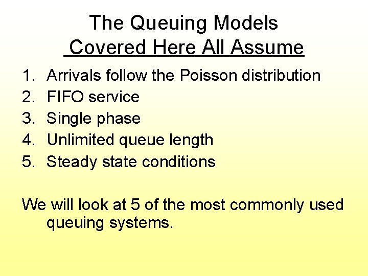
The Queuing Models Covered Here All Assume 1. 2. 3. 4. 5. Arrivals follow the Poisson distribution FIFO service Single phase Unlimited queue length Steady state conditions We will look at 5 of the most commonly used queuing systems.

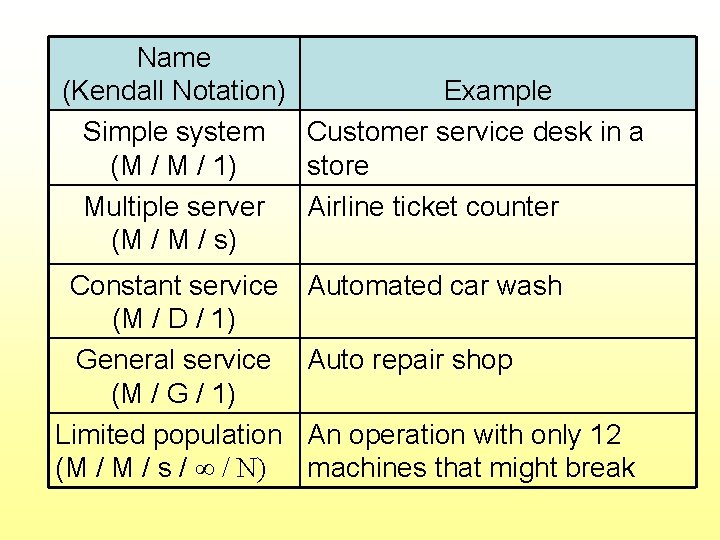
Name Models Covered (Kendall Notation) Example Simple system Customer service desk in a (M / 1) store Multiple server Airline ticket counter (M / s) Constant service (M / D / 1) General service (M / G / 1) Limited population (M / s / ∞ / N) Automated car wash Auto repair shop An operation with only 12 machines that might break

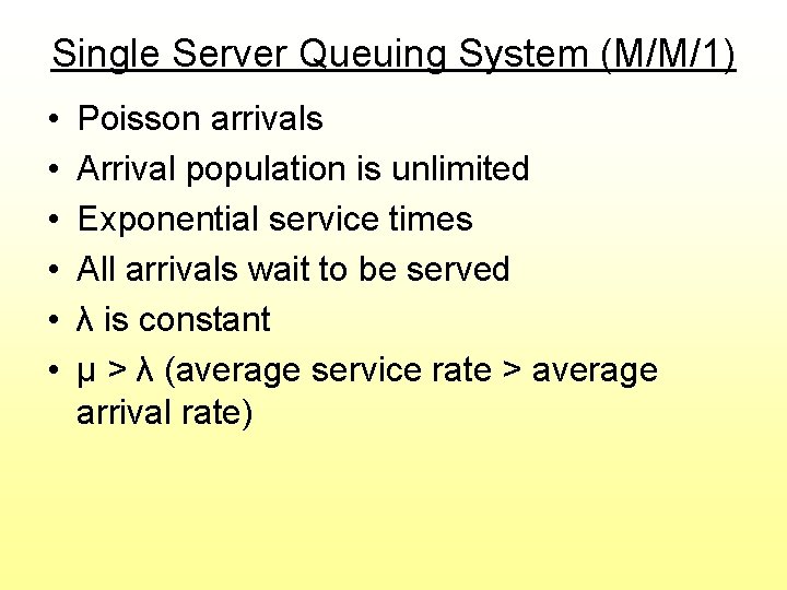
Single Server Queuing System (M/M/1) • • • Poisson arrivals Arrival population is unlimited Exponential service times All arrivals wait to be served λ is constant μ > λ (average service rate > average arrival rate)

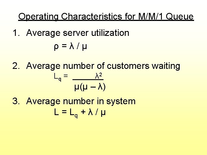
Operating Characteristics for M/M/1 Queue 1. Average server utilization ρ=λ/μ 2. Average number of customers waiting Lq = λ 2 μ(μ – λ) 3. Average number in system L = Lq + λ / μ

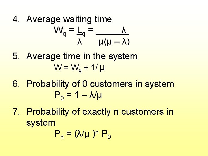
4. Average waiting time W q = Lq = λ λ μ(μ – λ) 5. Average time in the system W = Wq + 1/ μ 6. Probability of 0 customers in system P 0 = 1 – λ/μ 7. Probability of exactly n customers in system Pn = (λ/μ )n P 0

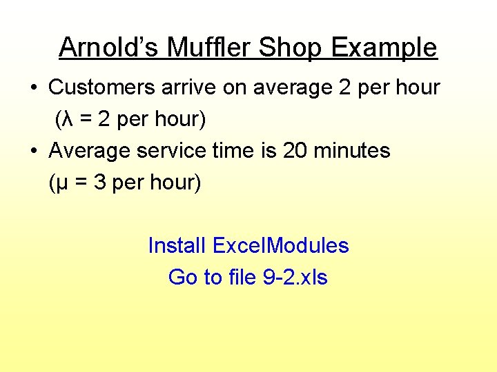
Arnold’s Muffler Shop Example • Customers arrive on average 2 per hour (λ = 2 per hour) • Average service time is 20 minutes (μ = 3 per hour) Install Excel. Modules Go to file 9 -2. xls

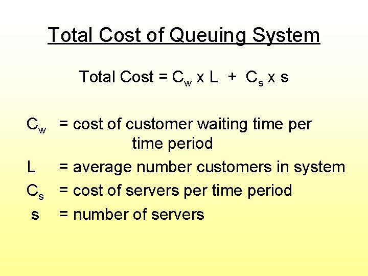
Total Cost of Queuing System Total Cost = Cw x L + Cs x s Cw = cost of customer waiting time period L = average number customers in system Cs = cost of servers per time period s = number of servers

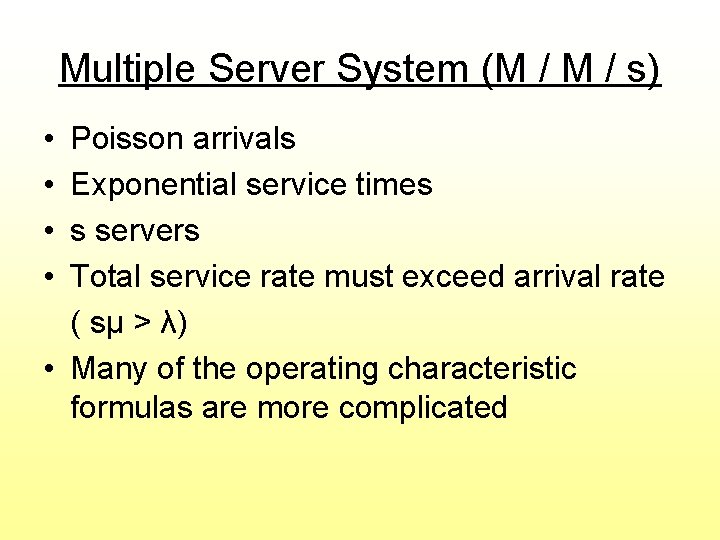
Multiple Server System (M / s) • • Poisson arrivals Exponential service times s servers Total service rate must exceed arrival rate ( sμ > λ) • Many of the operating characteristic formulas are more complicated

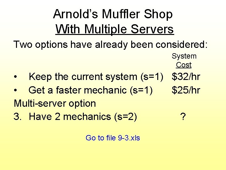
Arnold’s Muffler Shop With Multiple Servers Two options have already been considered: System Cost • Keep the current system (s=1) $32/hr • Get a faster mechanic (s=1) $25/hr Multi-server option 3. Have 2 mechanics (s=2) ? Go to file 9 -3. xls

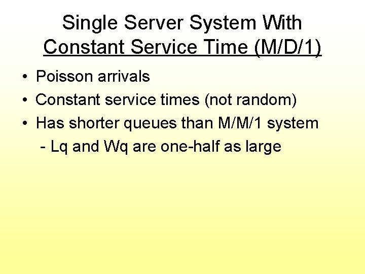
Single Server System With Constant Service Time (M/D/1) • Poisson arrivals • Constant service times (not random) • Has shorter queues than M/M/1 system - Lq and Wq are one-half as large

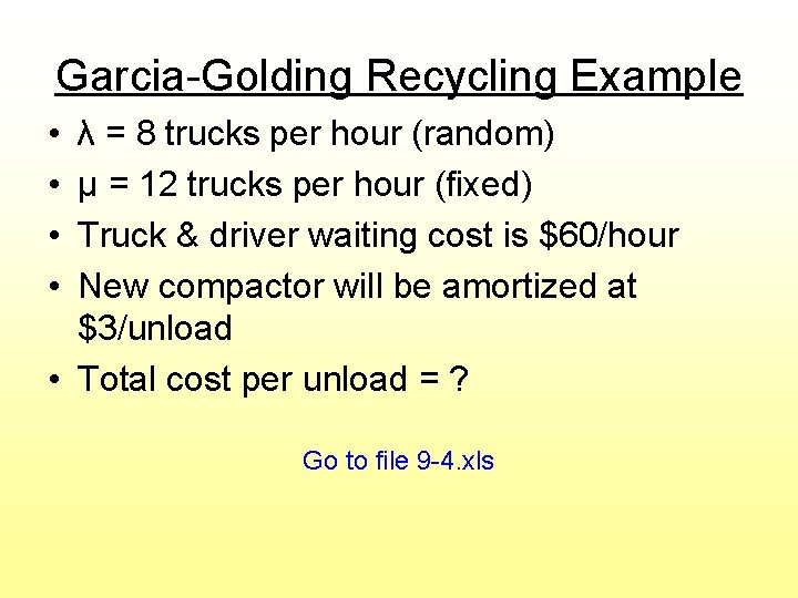
Garcia-Golding Recycling Example • • λ = 8 trucks per hour (random) μ = 12 trucks per hour (fixed) Truck & driver waiting cost is $60/hour New compactor will be amortized at $3/unload • Total cost per unload = ? Go to file 9 -4. xls

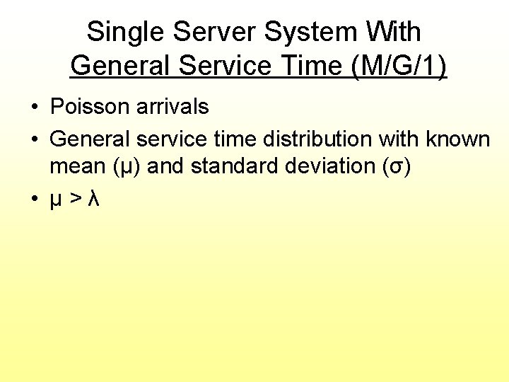
Single Server System With General Service Time (M/G/1) • Poisson arrivals • General service time distribution with known mean (μ) and standard deviation (σ) • μ>λ

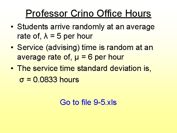
Professor Crino Office Hours • Students arrive randomly at an average rate of, λ = 5 per hour • Service (advising) time is random at an average rate of, μ = 6 per hour • The service time standard deviation is, σ = 0. 0833 hours Go to file 9 -5. xls

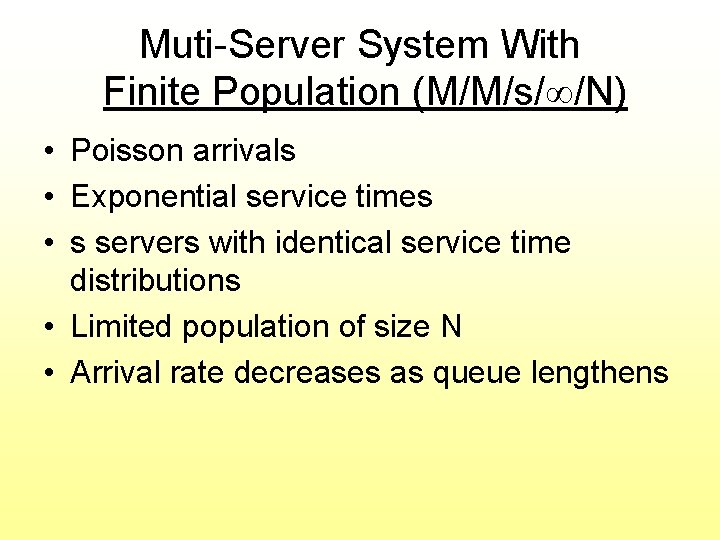
Muti-Server System With Finite Population (M/M/s/∞/N) • Poisson arrivals • Exponential service times • s servers with identical service time distributions • Limited population of size N • Arrival rate decreases as queue lengthens

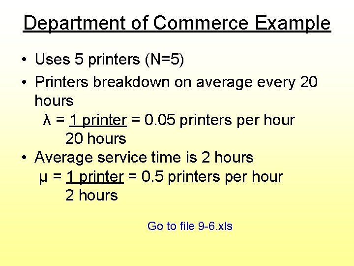
Department of Commerce Example • Uses 5 printers (N=5) • Printers breakdown on average every 20 hours λ = 1 printer = 0. 05 printers per hour 20 hours • Average service time is 2 hours μ = 1 printer = 0. 5 printers per hour 2 hours Go to file 9 -6. xls

More Complex Queuing Systems • When a queuing system is more complex, formulas may not be available • The only option may be to use computer simulation, which we will study in the next chapter