Proportional Hazards Model n Checking the adequacy of

Proportional Hazards Model n Checking the adequacy of the Cox model: n n n The functional form of a covariate The link function The validity of the proportional hazards assumptions 1

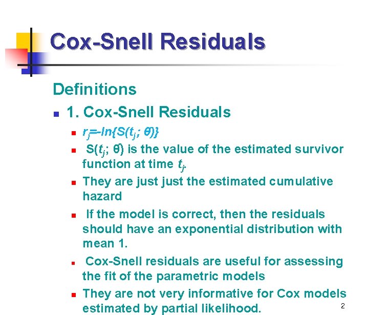
Cox-Snell Residuals Definitions n 1. Cox-Snell Residuals n n n rj=-ln{S(tj ; θ )} S(tj ; θ ) is the value of the estimated survivor function at time tj. They are just the estimated cumulative hazard If the model is correct, then the residuals should have an exponential distribution with mean 1. Cox-Snell residuals are useful for assessing the fit of the parametric models They are not very informative for Cox models 2 estimated by partial likelihood.

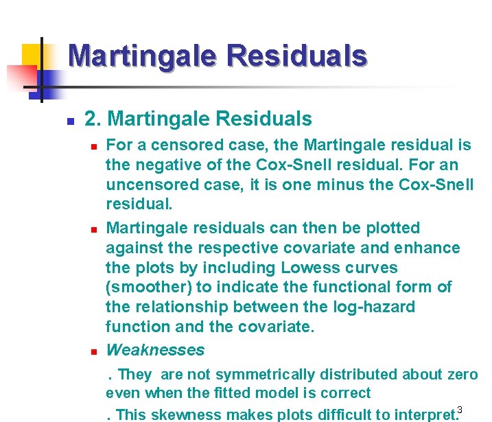
Martingale Residuals n 2. Martingale Residuals For a censored case, the Martingale residual is the negative of the Cox-Snell residual. For an uncensored case, it is one minus the Cox-Snell residual. n Martingale residuals can then be plotted against the respective covariate and enhance the plots by including Lowess curves (smoother) to indicate the functional form of the relationship between the log-hazard function and the covariate. n Weaknesses . They are not symmetrically distributed about zero n even when the fitted model is correct . This skewness makes plots difficult to interpret. 3

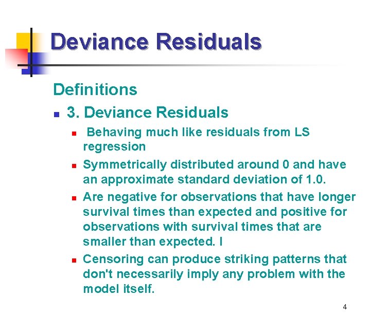
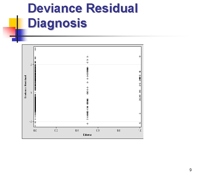
Deviance Residuals Definitions n 3. Deviance Residuals n n Behaving much like residuals from LS regression Symmetrically distributed around 0 and have an approximate standard deviation of 1. 0. Are negative for observations that have longer survival times than expected and positive for observations with survival times that are smaller than expected. I Censoring can produce striking patterns that don't necessarily imply any problem with the model itself. 4

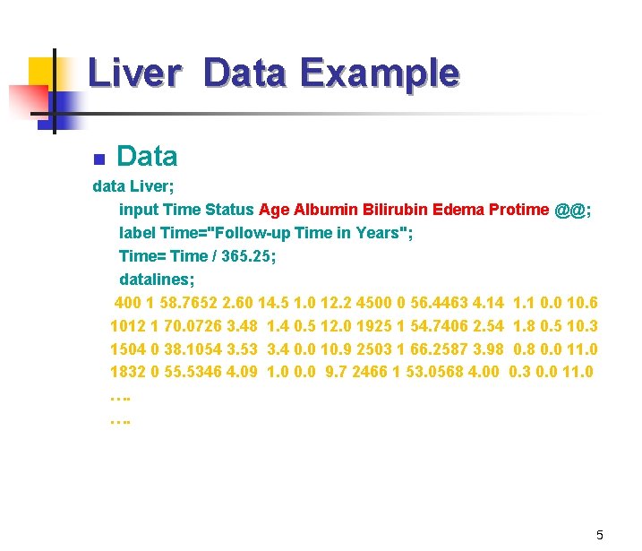
Liver Data Example n Data data Liver; input Time Status Age Albumin Bilirubin Edema Protime @@; label Time="Follow-up Time in Years"; Time= Time / 365. 25; datalines; 400 1 58. 7652 2. 60 14. 5 1. 0 12. 2 4500 0 56. 4463 4. 14 1. 1 0. 0 10. 6 1012 1 70. 0726 3. 48 1. 4 0. 5 12. 0 1925 1 54. 7406 2. 54 1. 8 0. 5 10. 3 1504 0 38. 1054 3. 53 3. 4 0. 0 10. 9 2503 1 66. 2587 3. 98 0. 0 11. 0 1832 0 55. 5346 4. 09 1. 0 0. 0 9. 7 2466 1 53. 0568 4. 00 0. 3 0. 0 11. 0 …. …. 5

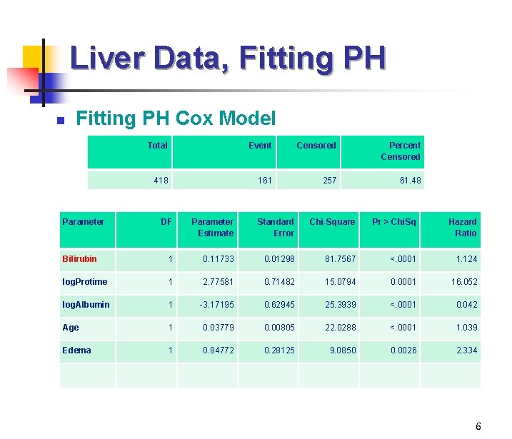
Liver Data, Fitting PH n Fitting PH Cox Model Parameter Total Event Censored Percent Censored 418 161 257 61. 48 DF Parameter Estimate Standard Error Chi-Square Pr > Chi. Sq Hazard Ratio Bilirubin 1 0. 11733 0. 01298 81. 7567 <. 0001 1. 124 log. Protime 1 2. 77581 0. 71482 15. 0794 0. 0001 16. 052 log. Albumin 1 -3. 17195 0. 62945 25. 3939 <. 0001 0. 042 Age 1 0. 03779 0. 00805 22. 0288 <. 0001 1. 039 Edema 1 0. 84772 0. 28125 9. 0850 0. 0026 2. 334 6

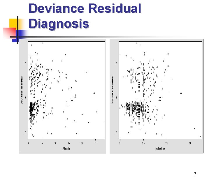
Deviance Residual Diagnosis 7

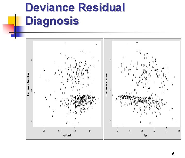
Deviance Residual Diagnosis 8

Deviance Residual Diagnosis 9

Conventional Residuals Analysis Issues highly subjective n difficult to interpret n 10

New Method of Residual Diagnosis n n n Objective way Checking model fit based on cumulative sumof Martingale Asymptotic property of the sum Gaussian Process Bootstrapping 11

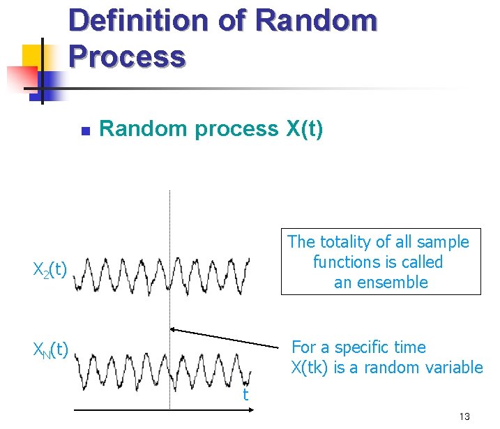
Definition of Random Process Definitions n 1. Random Process (Stochastic Process) n n A random process is the counterpart to a deterministic process. Instead of dealing with only one possible "reality" of how the process might evolve under time (as is the case, for example, for solutions of an ordinary differential equation), in a stochastic or random process there is some indeterminacy in its future evolution described by probability distributions This means that even if the initial condition (or starting point) is known, there are many possibilities the process might go to, but some paths are more probable and others less 12 Example: Markov process, , Gaussian process

Definition of Random Process n Random process X(t) X 2(t) The totality of all sample functions is called an ensemble XN(t) For a specific time X(tk) is a random variable t 13

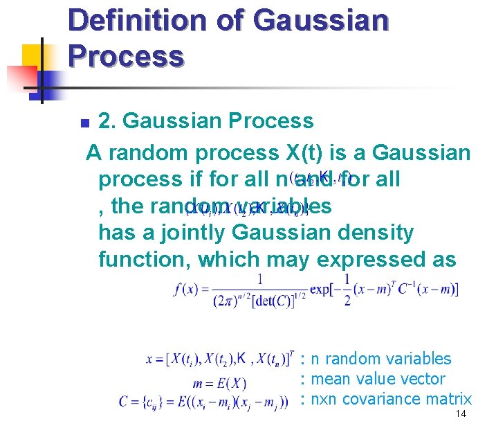
Definition of Gaussian Process 2. Gaussian Process A random process X(t) is a Gaussian process if for all n and for all , the random variables has a jointly Gaussian density function, which may expressed as n : n random variables : mean value vector : nxn covariance matrix 14

Why Gaussian Process ? n n Central limit theorem n The sum of a large number of independent and identically distributed(i. i. d) random variables getting closer to Gaussian distribution Cumulative residuals will be centered at zero if the model is correct. Under the null hypothesis of a correct model fit, they can be approximated as a zero mean Gaussian process with a covariance structure determined by the particular type of regression model. Realizations of the Gaussian process can be simulated by computer and compared with the observed process to assess whether the 15

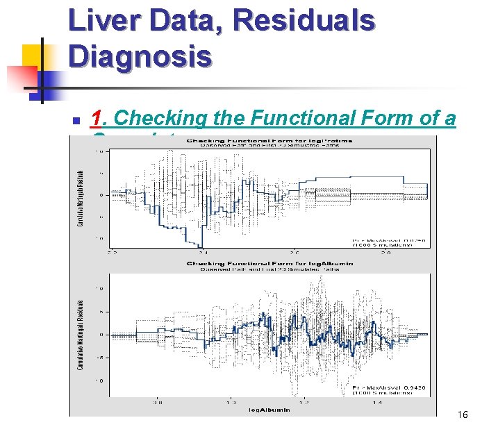
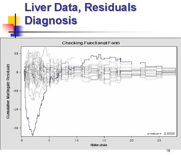
Liver Data, Residuals Diagnosis n 1. Checking the Functional Form of a Covariate 16

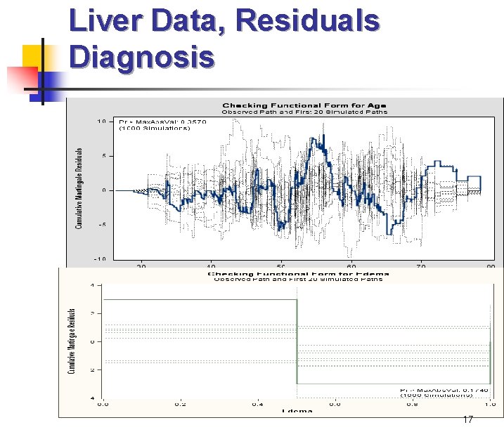
Liver Data, Residuals Diagnosis 17

Liver Data, Residuals Diagnosis 18

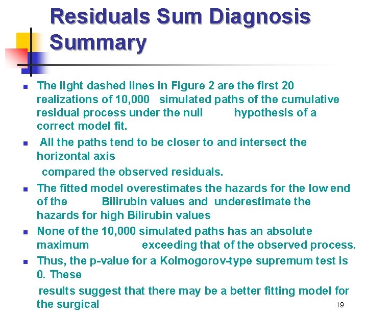
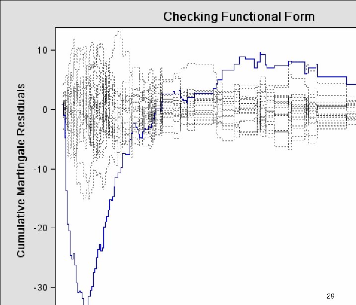
Residuals Sum Diagnosis Summary The light dashed lines in Figure 2 are the first 20 realizations of 10, 000 simulated paths of the cumulative residual process under the null hypothesis of a correct model fit. n All the paths tend to be closer to and intersect the horizontal axis compared the observed residuals. n The fitted model overestimates the hazards for the low end of the Bilirubin values and underestimate the hazards for high Bilirubin values n None of the 10, 000 simulated paths has an absolute maximum exceeding that of the observed process. n Thus, the p-value for a Kolmogorov-type supremum test is 0. These results suggest that there may be a better fitting model for 19 the surgical n

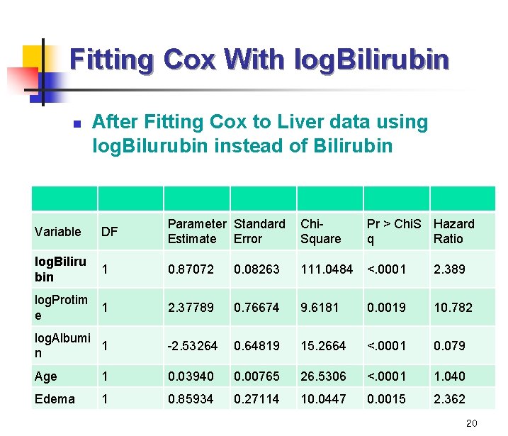
Fitting Cox With log. Bilirubin n After Fitting Cox to Liver data using log. Bilurubin instead of Bilirubin Variable DF Parameter Standard Estimate Error Chi. Square Pr > Chi. S Hazard q Ratio log. Biliru bin 1 0. 87072 0. 08263 111. 0484 <. 0001 2. 389 log. Protim 1 e 2. 37789 0. 76674 9. 6181 0. 0019 10. 782 log. Albumi 1 n -2. 53264 0. 64819 15. 2664 <. 0001 0. 079 Age 1 0. 03940 0. 00765 26. 5306 <. 0001 1. 040 Edema 1 0. 85934 0. 27114 10. 0447 0. 0015 2. 362 20

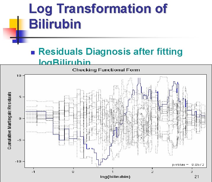
Log Transformation of Bilirubin n Residuals Diagnosis after fitting log. Bilirubin 21

Comment When the log transform is applied to Bilirubin, the observed process appears to be more typical of the simulated processes. n The p-value, based on 10, 000 simulated samples, is 0. 0572, indicating a much improved model n 22

Checking PH Assumptions n 2. Checking Proportional Hazards Assumptions n To check the proportional hazards assumption the score process (which is a transformed partial sum process of the martingale residuals) is compared to the simulated processes under the null hypothesis that the proportional hazards assumption holds. 23

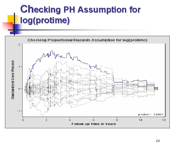
Checking PH Assumption for log(protime) 24

Comment n n The observed standardized score process for log(Protime) and the first 20 of 10, 000 simulated null processes reveals violation of the proportional hazards assumption As Lin et al. (1993) suggests, the violation may be corrected using time-dependent covariates or stratification 25

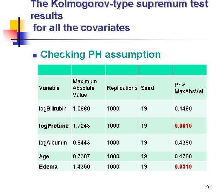
The Kolmogorov-type supremum test results for all the covariates n Checking PH assumption Variable Maximum Absolute Value Replications Seed Pr > Max. Abs. Val log. Bilirubin 1. 0880 1000 19 0. 1480 log. Protime 1. 7243 1000 19 0. 0010 log. Albumin 0. 8443 1000 19 0. 4390 Age 0. 7387 1000 19 0. 4780 Edema 1. 4350 1000 19 0. 0310 26

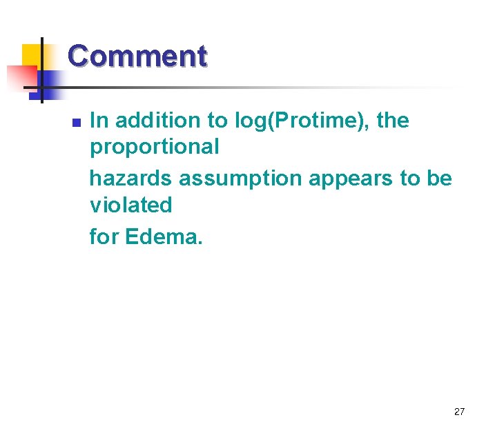
Comment In addition to log(Protime), the proportional hazards assumption appears to be violated for Edema. n 27

28

29