Model Checking II How CTL model checking works

Model Checking II How CTL model checking works

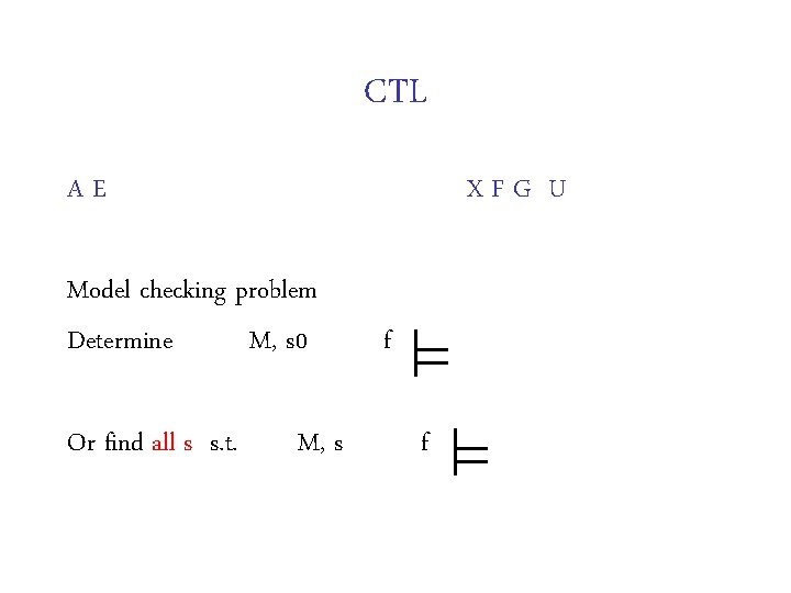
CTL AE XFG U Model checking problem Determine M, s 0 Or find all s s. t. M, s f f

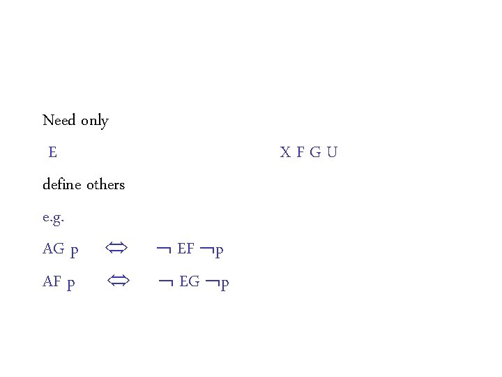
Need only E define others e. g. AG p AF p XFGU EF p EG p

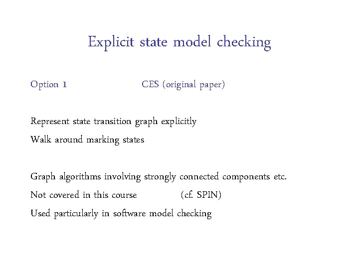
Explicit state model checking Option 1 CES (original paper) Represent state transition graph explicitly Walk around marking states Graph algorithms involving strongly connected components etc. Not covered in this course (cf. SPIN) Used particularly in software model checking

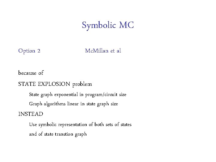
Symbolic MC Option 2 Mc. Millan et al because of STATE EXPLOSION problem State graph exponential in program/circuit size Graph algorithms linear in state graph size INSTEAD Use symbolic representation of both sets of states and of state transtion graph

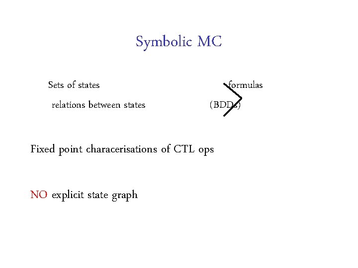
Symbolic MC Sets of states relations between states formulas (BDDs) Fixed point characerisations of CTL ops NO explicit state graph

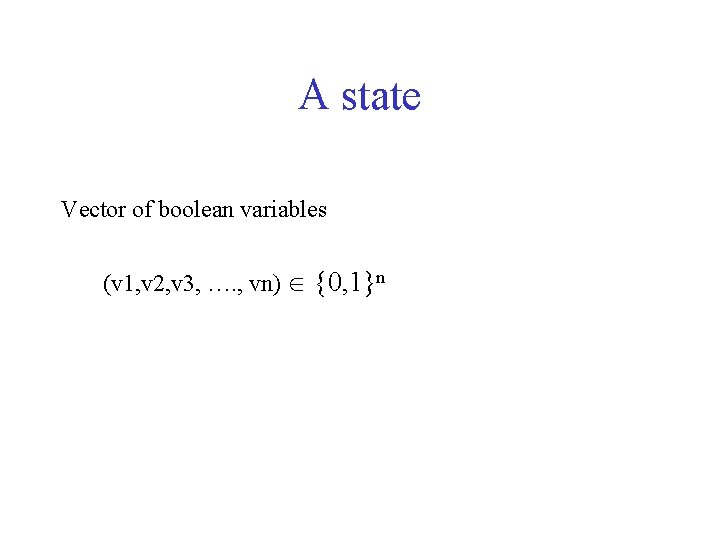
A state Vector of boolean variables (v 1, v 2, v 3, …. , vn) {0, 1}n

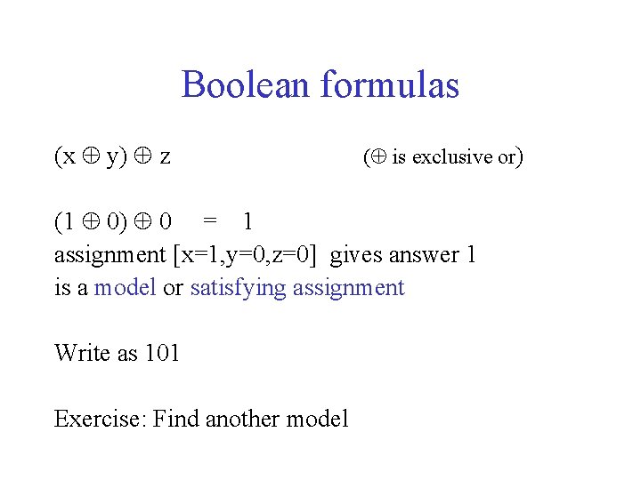
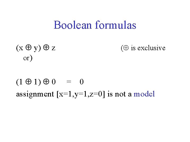
Boolean formulas (x y) z ( is exclusive or) (1 0) 0 = 1 assignment [x=1, y=0, z=0] gives answer 1 is a model or satisfying assignment Write as 101 Exercise: Find another model

Boolean formulas (x y) z or) ( is exclusive (1 1) 0 = 0 assignment [x=1, y=1, z=0] is not a model

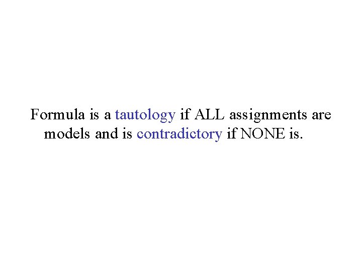
Formula is a tautology if ALL assignments are models and is contradictory if NONE is.

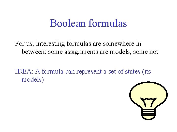
Boolean formulas For us, interesting formulas are somewhere in between: some assignments are models, some not IDEA: A formula can represent a set of states (its models)

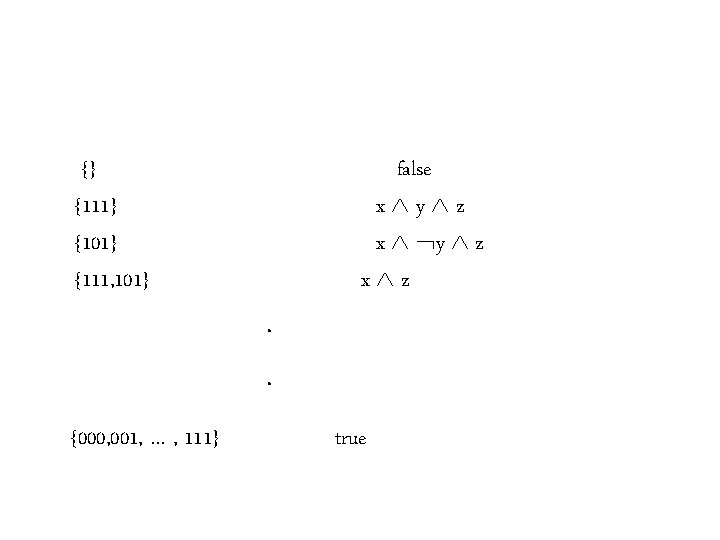
{} {111} {101} {111, 101} false x y z x y z x z . . {000, 001, … , 111} true

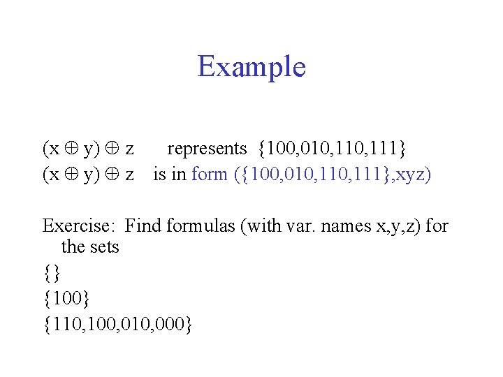
Example (x y) z represents {100, 010, 111} is in form ({100, 010, 111}, xyz) Exercise: Find formulas (with var. names x, y, z) for the sets {} {100} {110, 100, 010, 000}

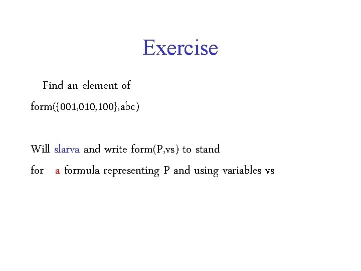
Exercise Find an element of form({001, 010, 100}, abc) Will slarva and write form(P, vs) to stand for a formula representing P and using variables vs

What is needed now? A good data structure for boolean formulas Binary Decision Diagrams (BDDs) Akers (IEEE Trans. Comp 78) Bryant (IEEE Trans. Comp. 86, most cited CS paper!) see also Bryant’s document about a Hitachi patent from 93 Mc. Millan saw application to symbolic MC

Binary Decision Diagrams Canonical form (constant time comparison) Polynomial algorithms for ’and’, ’or’, ’not’ etc. Exponential but practically efficient algorithm for boolean quantification (Presentation based on lecture notes by Ken Mc. Millan)

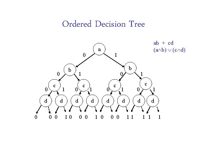
Ordered Decision Tree a 0 b 0 0 c d 0 1 d 0 0 0 c d 10 1 1 0 ab + cd (a b) (c d) 0 0 1 0 d d 1 0 c 0 0 b 1 1 0 d d 11 c 1 d 1 1 1

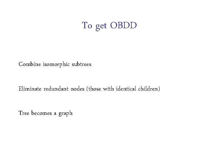
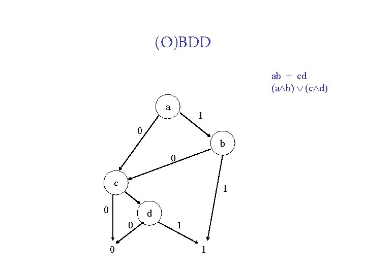
To get OBDD Combine isomorphic subtrees Eliminate redundant nodes (those with identical children) Tree becomes a graph

(O)BDD ab + cd (a b) (c d) a 1 0 b 0 c 1 0 d 0 0 1 1

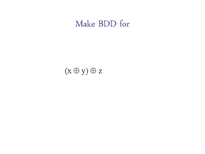
Make BDD for (x y) z

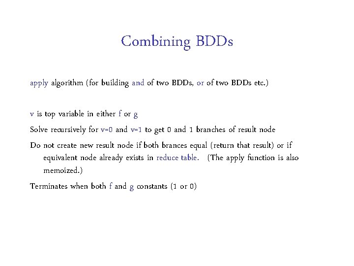
Combining BDDs apply algorithm (for building and of two BDDs, or of two BDDs etc. ) v is top variable in either f or g Solve recursively for v=0 and v=1 to get 0 and 1 branches of result node Do not create new result node if both brances equal (return that result) or if equivalent node already exists in reduce table. (The apply function is also memoized. ) Terminates when both f and g constants (1 or 0)

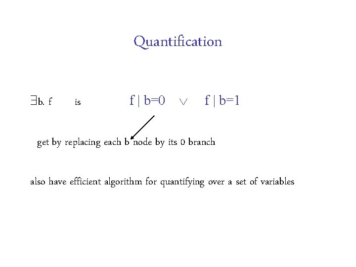
Quantification b. f is f | b=0 f | b=1 get by replacing each b node by its 0 branch also have efficient algorithm for quantifying over a set of variables

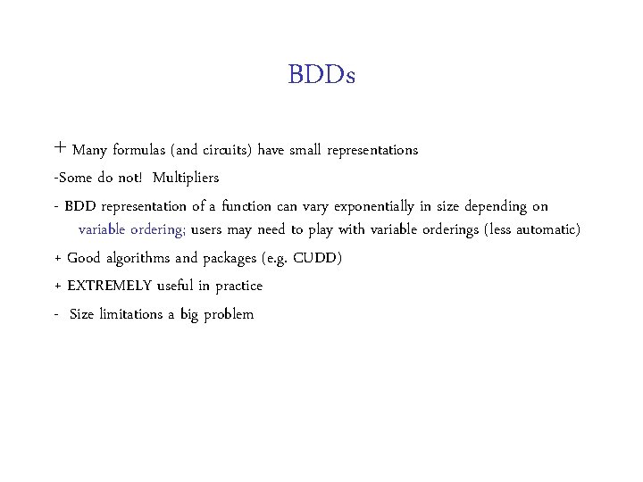
BDDs + Many formulas (and circuits) have small representations -Some do not! Multipliers - BDD representation of a function can vary exponentially in size depending on variable ordering; users may need to play with variable orderings (less automatic) + Good algorithms and packages (e. g. CUDD) + EXTREMELY useful in practice - Size limitations a big problem

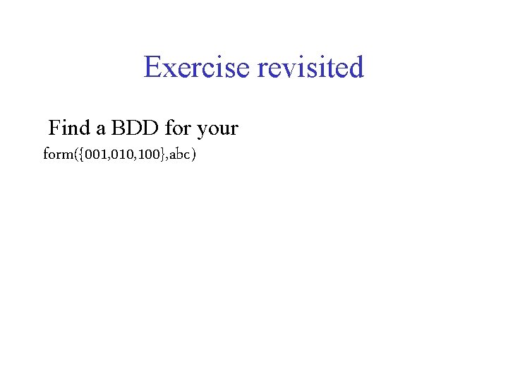
Exercise revisited Find a BDD for your form({001, 010, 100}, abc)

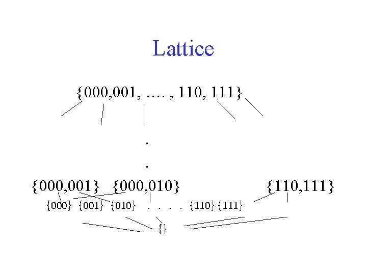
Lattice {000, 001, …. , 110, 111}. . {000, 001} {000, 010} {001} {010}. . {110} {111} {} {110, 111}

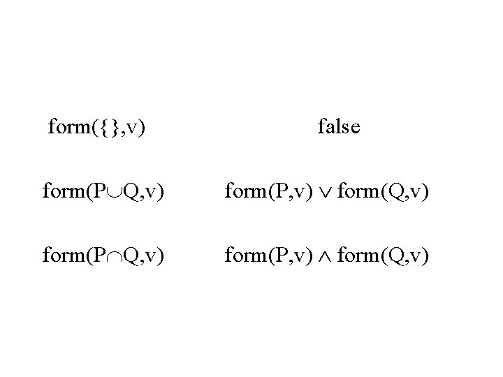
form({}, v) false form(P Q, v) form(P, v) form(Q, v)

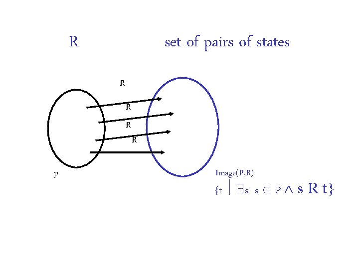
R set of pairs of states R R R p R Image(P, R) {t s s P s R t}

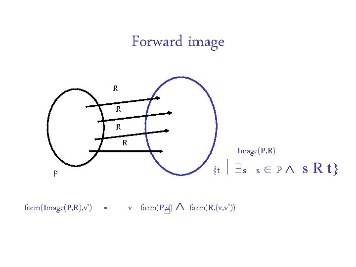
Forward image R R p form(Image(P, R), v’) = Image(P, R) {t s s P s R t} v form(P, v) form(R, (v, v’))

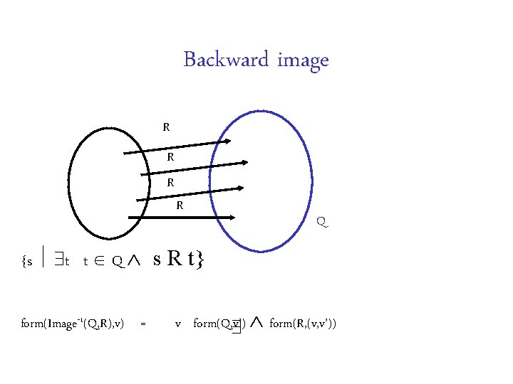
Backward image R R Q {s t t Q s R t} form(Image-1(Q, R), v) = v form(Q, v’) form(R, (v, v’))

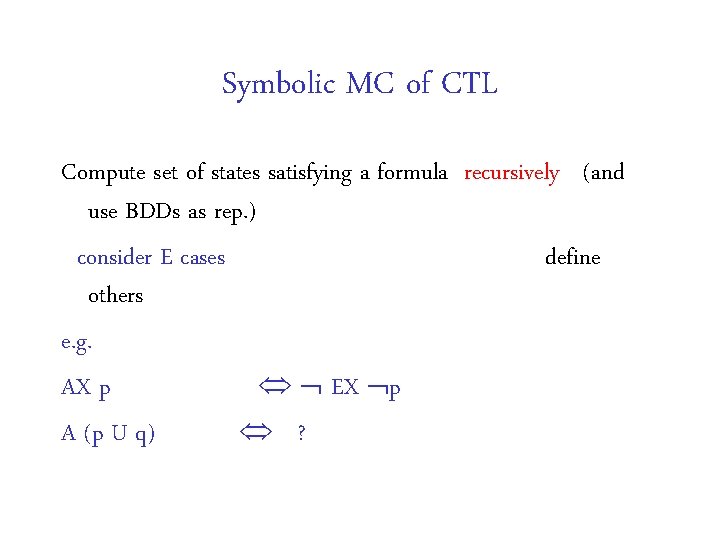
Symbolic MC of CTL Compute set of states satisfying a formula recursively (and use BDDs as rep. ) consider E cases define others e. g. AX p EX p A (p U q) ?

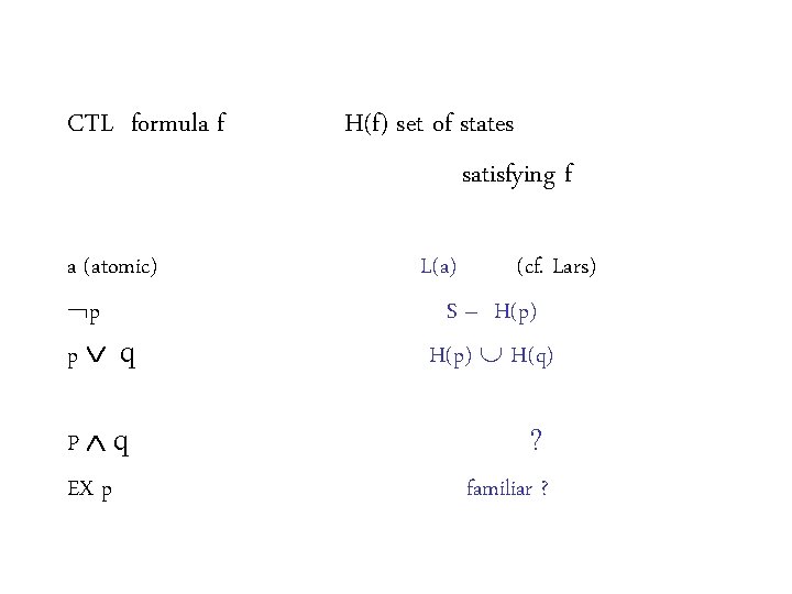
CTL formula f a (atomic) p p q P q EX p H(f) set of states satisfying f L(a) (cf. Lars) S – H(p) H(q) ? familiar ?

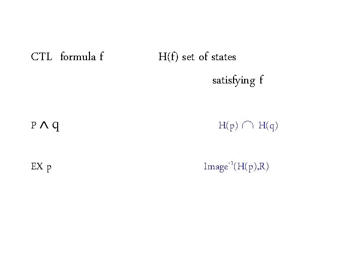
CTL formula f P q EX p H(f) set of states satisfying f H(p) H(q) Image-1(H(p), R)

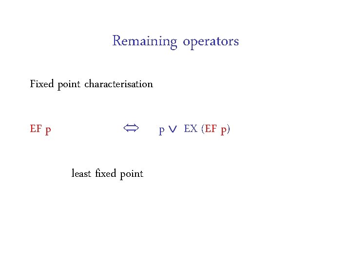
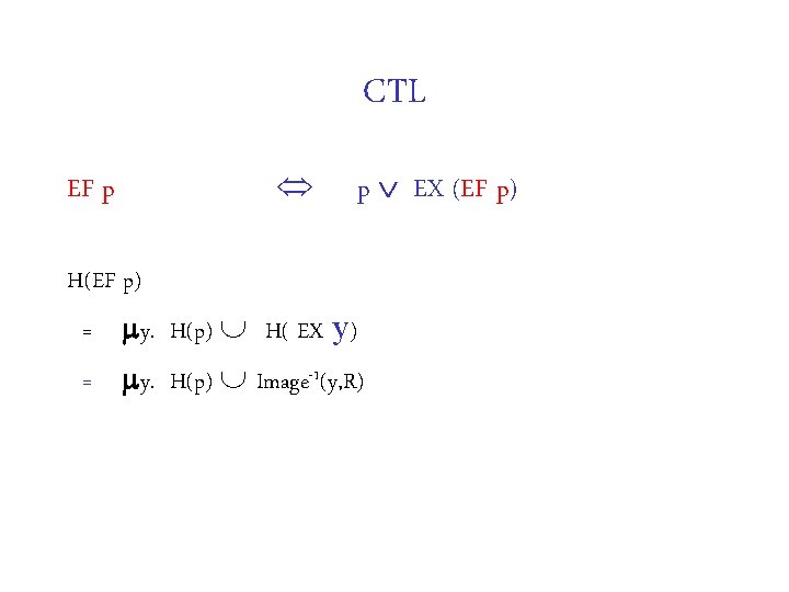
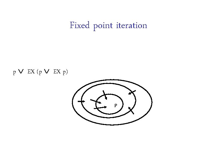
Remaining operators Fixed point characterisation EF p least fixed point p EX (EF p)

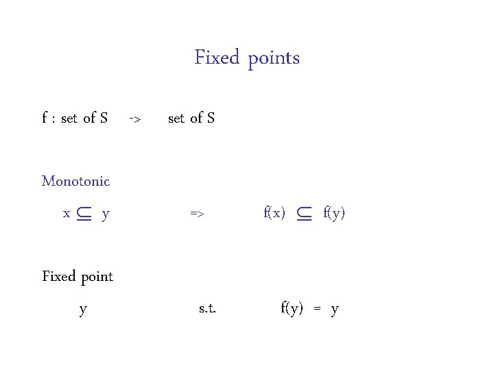
Fixed points f : set of S -> Monotonic x y Fixed point y set of S => s. t. f(x) f(y) = y

Fixed points monotonic f has Least fixed point y. f(y) [lfp y. f(y)] Greatest fixed point y. F(y) [gfp y. F(y)]

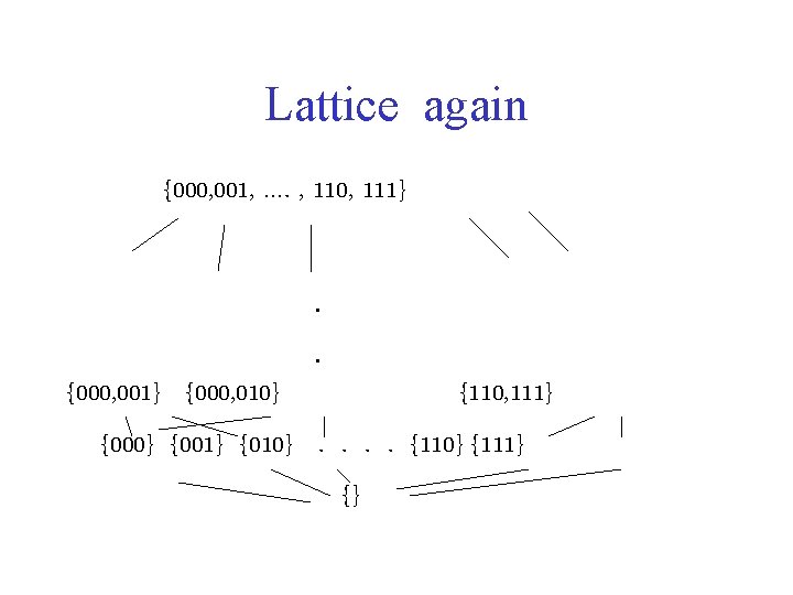
Lattice again {000, 001, …. , 110, 111}. . {000, 001} {000, 010} {110, 111} {000} {001} {010}. . {110} {111} {}

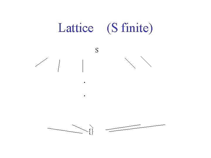
Lattice (S finite) S . . {}

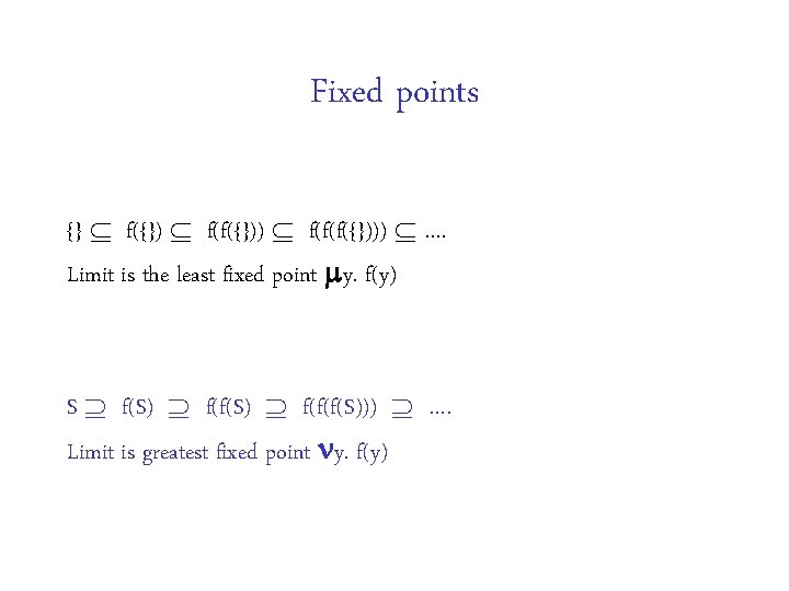
Fixed points {} f({}) f(f({})) f(f(f({}))) …. Limit is the least fixed point y. f(y) S f(S) f(f(f(S))) …. Limit is greatest fixed point y. f(y)

CTL EF p p EX (EF p) H(EF p) = y. H(p) H( EX y) = y. H(p) Image-1(y, R)

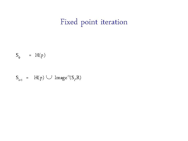
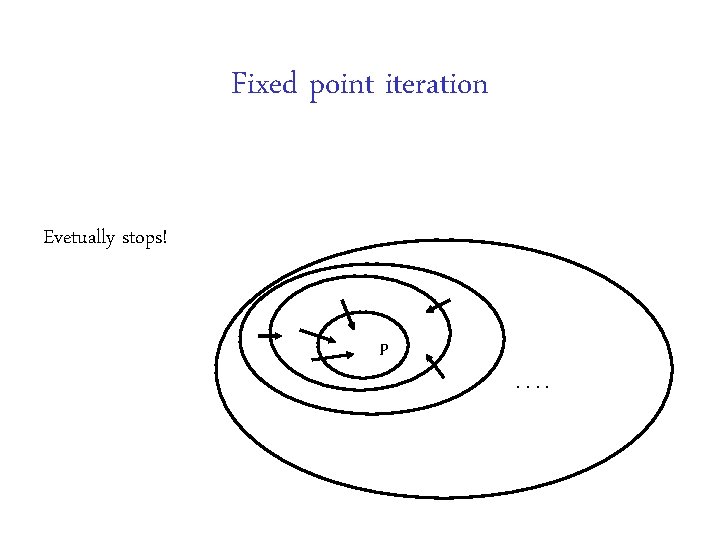
Fixed point iteration S 0 = H(p) Si+1 = H(p) Image-1(Si, R)

Fixed point iteration P

Fixed point iteration p EX (p EX p) P

Fixed point iteration Evetually stops! P. .

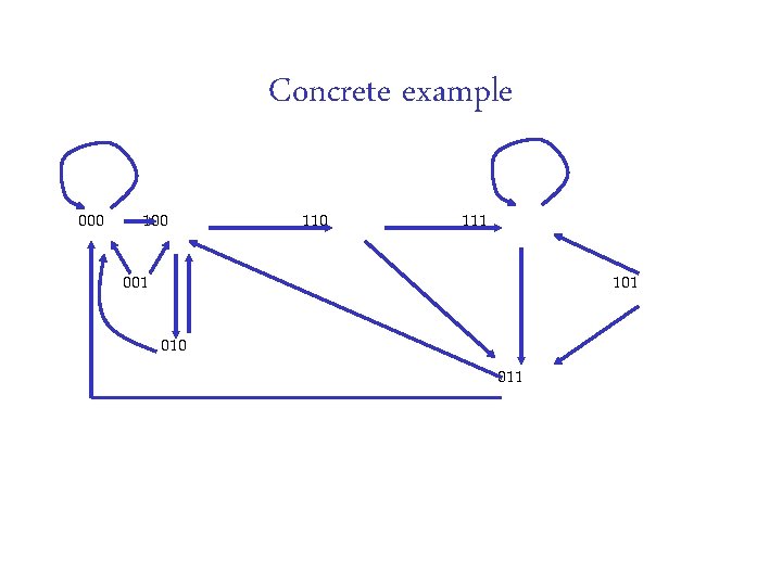
Concrete example 000 110 111 001 101 010 011

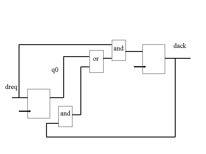
Concrete example 0 000 100 4 110 6 7 111 001 1 101 010 2 EF p 011 p = dreq q 0 dack 3 5

and or q 0 dreq and dack

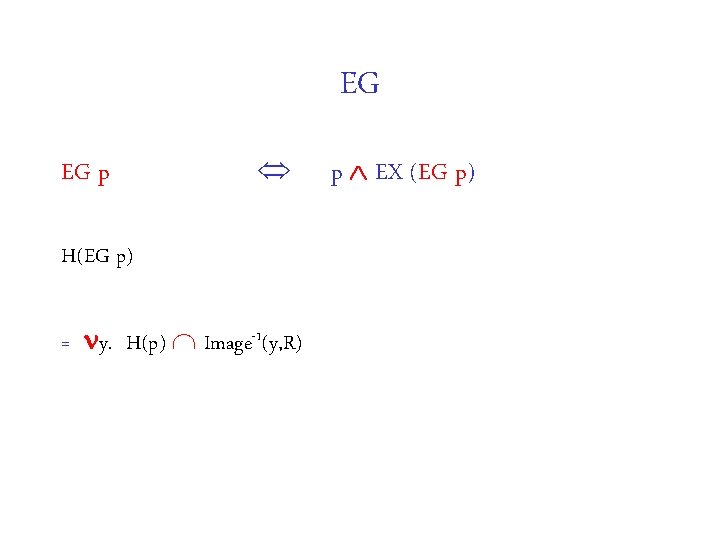
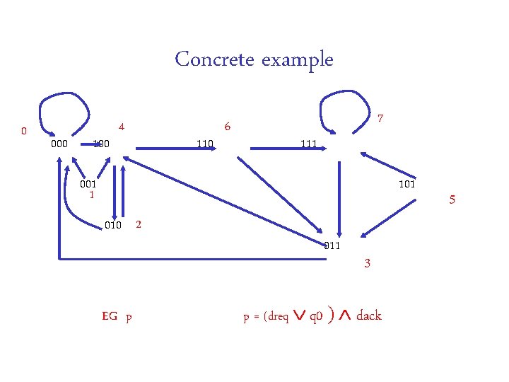
EG EG p H(EG p) = y. H(p) Image-1(y, R) p EX (EG p)

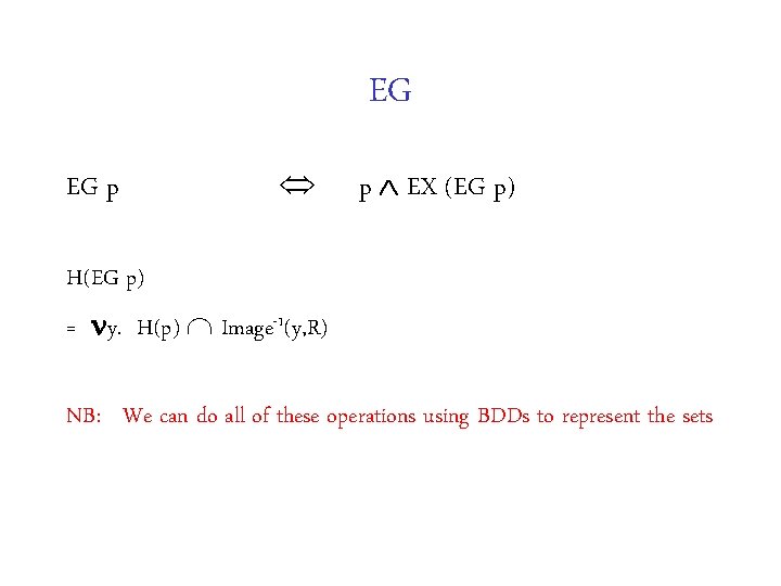
EG EG p p EX (EG p) H(EG p) = y. H(p) Image-1(y, R) NB: We can do all of these operations using BDDs to represent the sets

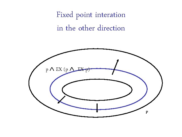
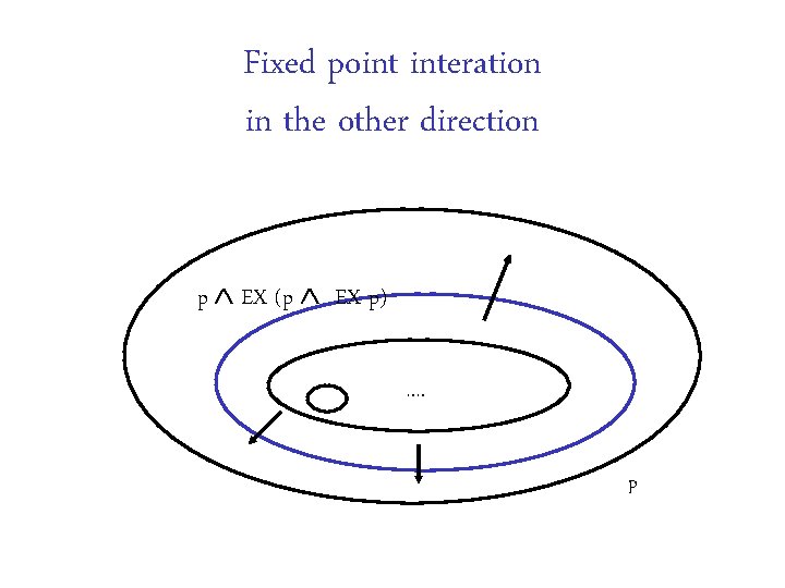
Fixed point interation in the other direction P

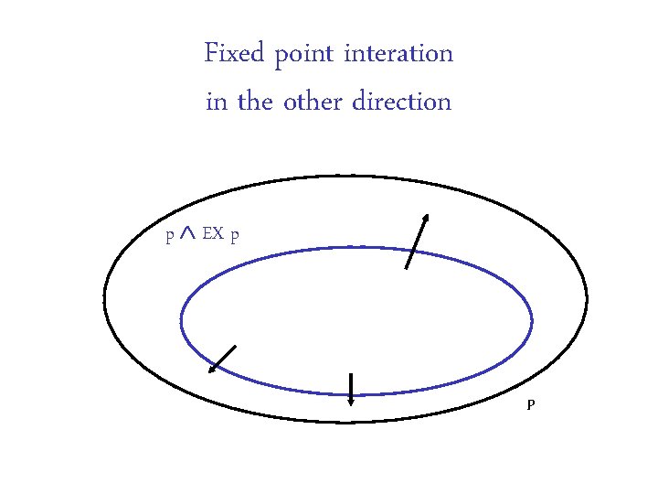
Fixed point interation in the other direction p EX p P

Fixed point interation in the other direction p EX (p EX p) P

Fixed point interation in the other direction p EX (p EX p) …. p

Concrete example 0 000 100 4 110 6 7 111 001 1 101 010 2 EG p 011 3 p = (dreq q 0 ) dack 5

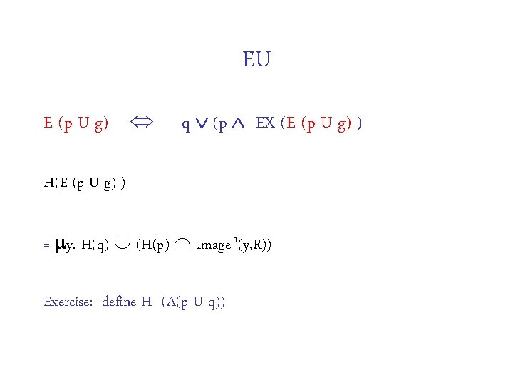
EU E (p U g) q (p EX (E (p U g) ) H(E (p U g) ) = y. H(q) (H(p) Image-1(y, R)) Exercise: define H (A(p U q))

All done with BDDS! Glad påsk