Contents CTL Model Checking Timed Automata TA Timed
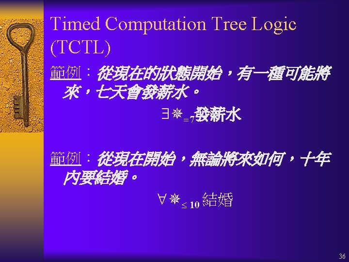
 ¨ Timed Computation Tree Logic")
 for f 1 U f 2 9")
 在M (剩餘的M)中,所有狀態都滿足φ。 執行 transitive closure: 1 For all s, s do if (s,")
 ¨ A strongly connected component (SCC) C is a maximal")
 for f 1 13")

 ¨ ◇(Start Heat) ¨ S(Start) = {2, 5,")

 ¨ (Start ◇Heat) ¨ F = { ◇(Start Close Error)}")
 ¨ Real-Time Properties:")


 s 0")
┝ φ1")
┝")


 ¨ Clock zones are closed under 3 operations: ¨ Let z")
 60")
, where s: location, z: clock zone")
) To obtain Successor Clock Zone (succ(z, e)) ¨ Intersect z")
 ¨ States = zones")
 ¨ DBM is a matrix to represent a clock zone")
 ¨ x 1 x 2 < 2 0 < x 2 2")
 ¨ A zone is not uniquely represented by a DBM ¨ Zone:")
 ¨ Canonical (unique) form of DBM for a zone ¨ Tightening")
 ¨ Check if all elements on main diagonal are ( 0) –")
 ¨ Intersection: D = D 1 D 2 (all DBMs)")
![DBM (3 operations: Clock Reset) D' = D [Y : = 0], Y X](https://slidetodoc.com/presentation_image_h/24e01352cd742e0863ba7a7e6a009402/image-70.jpg "DBM (3 operations: Clock Reset) D' = D [Y : = 0], Y X")
 ¨ Time Elapse: D' = te(D) defined as follows:")
 ¨ All 3 operations can be efficiently implemented ¨ DBM must")
 ¨ Clock zones: represented by DBM ¨ Succesor clock zones")
 ¨ Initial state: (s 0, Z 0), Z 0: x")
 ¨ Invariant (s 0) is 0≤x 0≤y≤ 5 75")
 ¨ Step 1: Intersection D 0 with (s 0) gives")
 ¨ Step 3: Intersect with (s 0) again 77")
 ¨ Trigger (a) = y 3 78")
 ¨ Step 4: Intersect with trigger (a) 79")
 ¨ Step 5: Reset clock y in DBM Z 1")
 ¨ Successor of (s 0, Z 0) is (s 1,")
 ¨ BDD: A canonical form representation for Boolean formulas. ¨")
 83")
 ¨ Binary Decision Trees (BDT): – Same size as truth")
 ¨ BDD B with root v determines Boolean function fv(x 1,")
 ¨ Canonical Form: Two boolean functions are logically equivalent iff they")
 ¨ For requirement 1 (same variable order): – Total ordering <")
 ¨ Remove duplicate terminals: Eliminate all but one terminal vertex with")
 ¨ Apply 3 transformations repeatedly in a bottom-up manner ¨ Time:")
 ¨ Since OBDDs are canonical, it is easy to: – check")
 ¨ a 1 < a 2 < b 1 < b")
 ¨ Infeasible to find an optimal variable ordering! ¨ Checking a")
 ¨ Heuristics to find a good variable ordering: ¨ Depth-First Traversal")
 ¨ All 16 two-argument logical operations can be implemented efficiently on OBDDs.")
 ¨ If v, v' are terminals, f * f ' =")
 ¨ A problem generates 2 sub-problems ¨ Use dynamic programming to avoid")
 ¨ State variables: a, b ¨ Add new state variables:")

: Finite Kripke Structure ¨ P(S): power set of")

 2(False) … ¨ No. of iterations |S| ¨ Last")

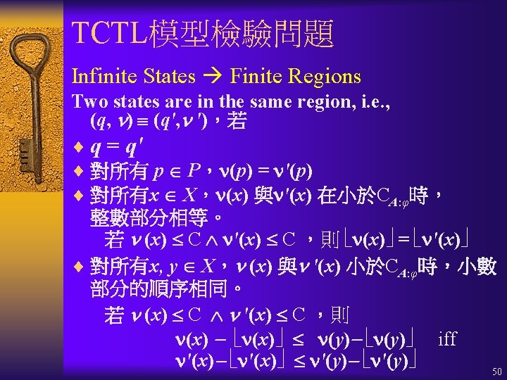
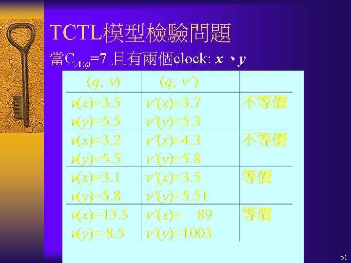
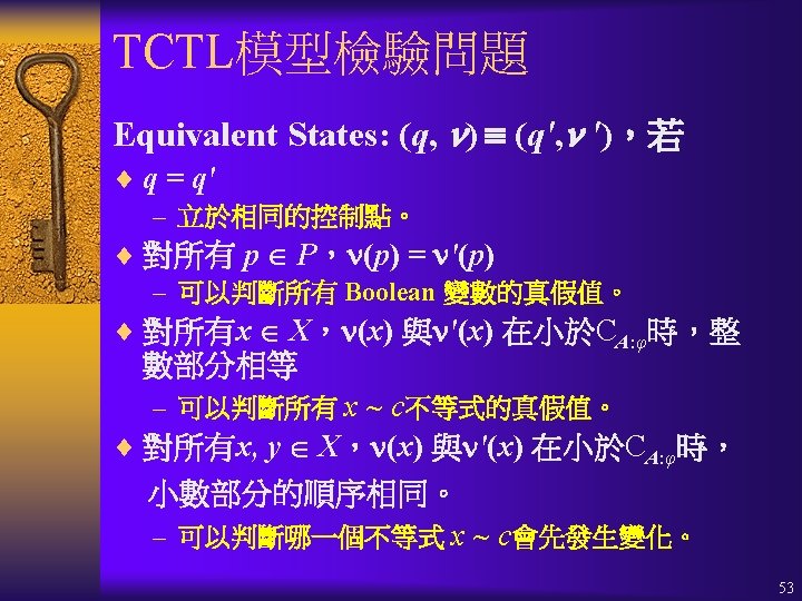
 2(True) … ¨ No. of iterations |S| ¨ Last")


![Approximations for [p U q] 106](https://slidetodoc.com/presentation_image_h/24e01352cd742e0863ba7a7e6a009402/image-106.jpg "Approximations for [p U q] 106")

 returns an OBDD that represents all")
 = Check. EX(Check(f )) ¨ Check(")
 ¨ f is true in a state if it has a")
![Check. EU(f ) ¨ Least fixpoint characterization: [ 1 U 2] = Z. 2](https://slidetodoc.com/presentation_image_h/24e01352cd742e0863ba7a7e6a009402/image-111.jpg "Check. EU(f ) ¨ Least fixpoint characterization: [ 1 U 2] = Z. 2")
 ¨ Greatest fixpoint characterization = Z. Z ¨ Use Gfp() to")


, where each node in V is an")


 ¨ Use n operator")
 ¨ ((stall destaddr)")
 ¨ 8 -bit wide pipeline ¨ 4 general registers")
- Slides: 125
Contents ¨ CTL Model Checking ¨ Timed Automata (TA) ¨ Timed Computation Tree Logic (TCTL) ¨ TCTL Model Checking ¨ Clock Zones, DBM, BDD ¨ Symbolic Model Checking ¨ Counterexample & Witnesses 2
Check. EU(f 1, f 2) for f 1 U f 2 9
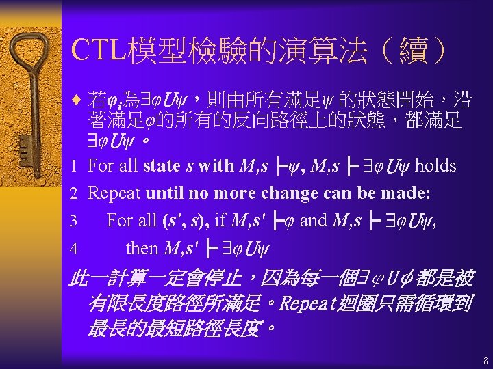
CTL模型檢驗的演算法(續) 在M (剩餘的M)中,所有狀態都滿足φ。 執行 transitive closure: 1 For all s, s do if (s, s ) M , Reach[s, s ] : = 1; else Reach[s, s ] : = 0; 2 For s, s do For all s do Reach[s, s ] : = Reach[s, s ] (Reach[s, s ] Reach[s , s ]); 11
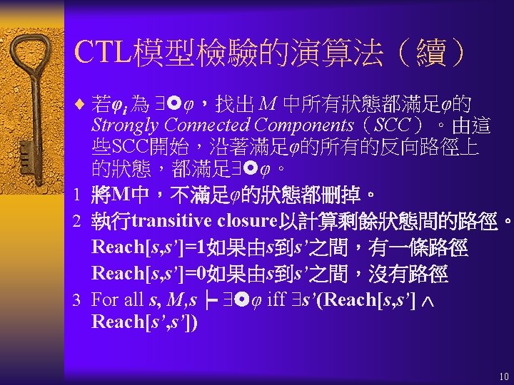
Strongly Connected Components (SCC) ¨ A strongly connected component (SCC) C is a maximal sub-graph such that every node in C is reachable from every other node in C along a directed path entirely contained within C. s 1 s 2 Two SCC: {s 1, s 2, s 3} {s 4} s 4 s 3 s 5 12
Check. EG( f 1) for f 1 13
Microwave Oven Example 14
Microwave Oven Example ¨ (Start ◇Heat) ¨ ◇(Start Heat) ¨ S(Start) = {2, 5, 6, 7} ¨ S( Heat) = {1, 2, 3, 5, 6} ¨ SCC( Heat) = {1, 2, 3, 5} ¨ S(Start Heat) = {2, 5} ¨ S( ◇(Start Heat)) = {1, 2, 3, 4, 5, 6, 7} ¨ S( ◇(Start Heat)) = 15
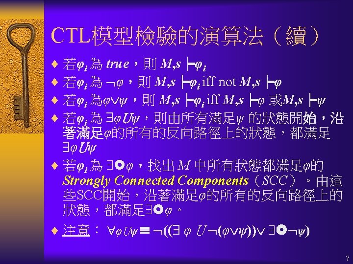
Fairness Constraints ¨ F = {P 1, …, Pk} // fairness constraints ¨ Fair SCC C Pi F, state ti (C Pi). ¨ Check. Fair. EG(f 1): Fair SCCs ¨ Define “fair”: atomic proposition, true at a state s iff there is a fair path starting at s. ¨ M, s┝ p fair, M, s┝ (f 1 fair), ¨ Check. EUFair(f 1, f 2) = Check. EU(f 1, f 2 fair) = M, s┝ (f 1 U (f 2 fair)) 16
Microwave Oven (with Fairness) ¨ (Start ◇Heat) ¨ F = { ◇(Start Close Error)} ¨ S(Start) = {2, 5, 6, 7} ¨ S( Heat) = {1, 2, 3, 5, 6} ¨ SCC( Heat) = {1, 2, 3, 5} is NOT fair ¨ S( Heat) = { } ¨ S( ◇(Start Heat))={1, 2, 3, 4, 5, 6, 7} 17
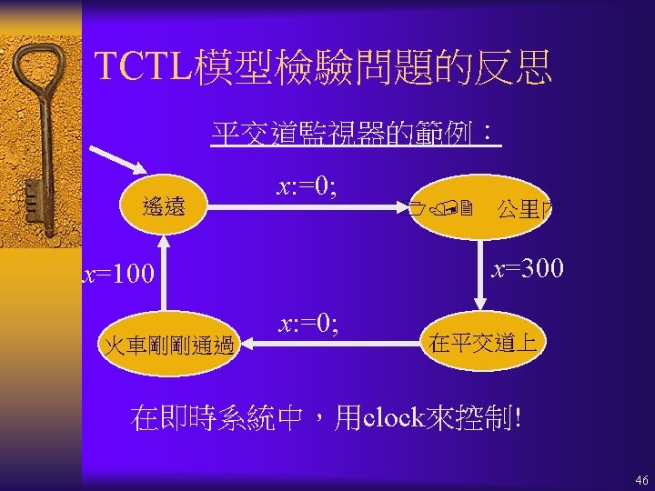
Model Checking Real-Time Systems ¨ Real-Time Systems: – Timed Automata (TA) ¨ Real-Time Properties: – Timed Computation Tree Logic (TCTL) ¨ Given a real-time system S modeled by a set of TA {A 1, A 2, …, An} and a real-time property specified by a TCTL formula , check if S satisfies (S┝ ? ). 18
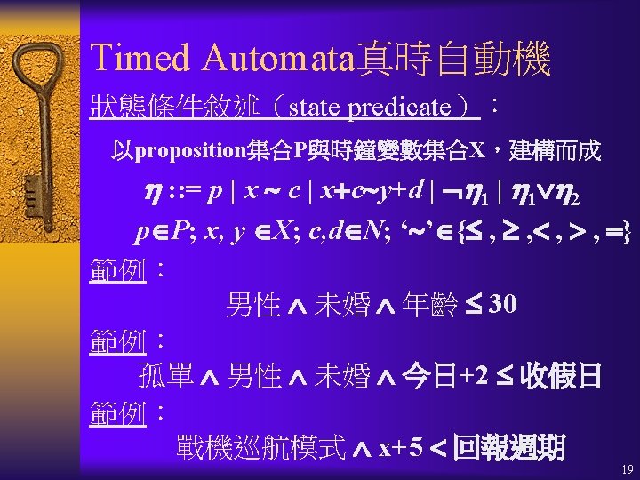
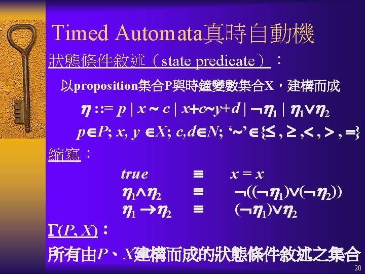
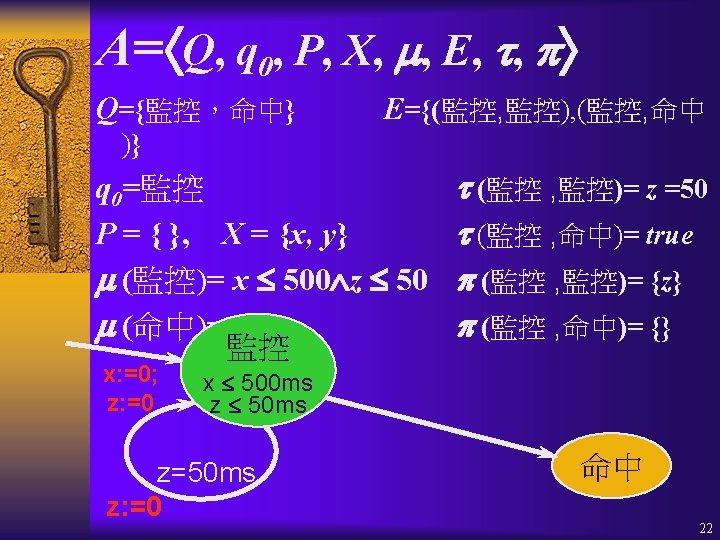
Timed Automata真時自動機 A = Q, q 0, P, X, , E, , Q : 有限控制點的集合 (set of control locations) q 0 : 啟始控制點 (initial location) P : 命題的集合 (set of propositions) X : 時鐘變數的集合 (set of clock variables) : Q (P, X);各控制點的恆定條件 (invariant) E Q Q : 控制點轉換的集合 (set of transitions) : E (P, X);各轉換的激發條件 (triggering condition) : E 2 X : 在轉換時,要被reset成零(歸零)的 時鐘變數的集合 (set of clocks to be reset) 21
Parallel Composition of TA ¨ A 1= Q 1, q 01, P 1, X 1, E 1, 1 , A 2= Q 2, q 02, P 2, X 2, E 2, 2 ¨ A 1 ∥A 2 = Q 1 Q 2, q 0, P 1 P 2 X 1 X 2 , E, 1 2 ¨ q 0: a merge of q 01 and q 02 ¨ (q, q') = 1(q) 2(q') ¨ E: set of interleaved transitions with synchronization transitions identified 23
A Manufacturing Example 24
Manufacturing Ex: D-Robot TA 25
Manufacturing Ex: G-Robot TA 26
Manufacturing Ex: Station TA 27
Manufacturing Ex: Box TA 28
Model of Manufacturing System ¨ M = D-Robot || G-Robot || Station || Box ¨ Transitions with same labels are identified as one in M. ¨ E. g. : g-put in G-Robot, Station, and Box ¨ E. g. : d-pick in D-Robot, Station, and Box 29
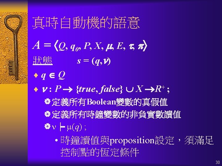
真時自動機的語意 A= Q, q 0, P, X, , E, , 的計算 (computation) s 0 -run: s 0 s 1 s 2. . . sk. . ¨ 對所有k 0, sk 是具有如(q, )格式的狀態。 ¨ 存在一個monotonically increasing、 divergent的非負實數序列 t 0 t 1 t 2. . . tk. . 對所有k 0, u對所有 t [0, tk+1 tk ], sk t┝ (q) u. Either sk (tk+1 tk ) = sk+1 or sk (tk+1 tk ) sk+1 35
TCTL的語意 A= Q, q 0, P, X, , E, , A, (q, )┝ φ1 U cφ2 iff 存在 ¨ (q, )-run:s 0 s 1 s 2. . . sk. . ,與 ¨ monotonically increasing、divergent的非負 實數序列:t 0 t 1 t 2. . . 與 ¨ k 0,與 t [0, tk+1 tk], utk+t t 0 c u. A, sk+t┝φ2 u對所有k h 0與 t’ [0, th+1 th], A, sh+t’┝φ1 u對所有 t’ [0 , t),A, sk+t’┝φ1 42
TCTL的語意 A = Q, q 0, P, X, , E, , A, (q, )┝ cφ1 iff 存在 ¨ (q, )-run:s 0 s 1 s 2. . . sk. . ,與 ¨ monotonically increasing、divergent的非 負實數序列:t 0 t 1 t 2. . . 對所有k 0,與 t [0, tk+1 tk], 若 tk+t t 0 c,則 A, sk+t┝φ1 43
2 Clocks with cx= 2, cy= 1 28 Clock Regions: • 6 corner points, • 14 open line segments, • 8 open regions 52
TCTL的驗證問題複雜度 ¨ TCTL與真時自動機的模型檢驗問題是 PSPACE-complete。 ¨ TCTL的satisfiability問題,是undecidable。 57
Clock Zones ¨ Finite representation of infinite state-space ¨ Conjunction of inequalities such as: x<c | x≤c | x–y<c | x–y≤c x, y X, c Z ¨ General form of a clock zone: x 0 = 0 0 i j n (xi – xj ~ cij) ~ {< , ≤} 58
Clock Zones (Operations) ¨ Clock zones are closed under 3 operations: ¨ Let z 1, z 2 be two clock zones, Y X, t 0 ¨ Intersection: z 1 z 2 is a clock zone (Conjunction of conjunctions) ¨ Clock Reset: z 1(Y: =0) is a clock zone (Proof on pages 284 ~ 287) ¨ Time Elapse: z 1 + t is a clock zone (See next page) 59
Clock Zones (Time Elapse) 60
Zones = Symbolic States ¨ Zone: (s, z), where s: location, z: clock zone represents a symbolic state. ¨ Successor Clock Zone: z' = succ(z, e), where z: clock zone, e: transition (successor clock zone obtained from z after time elapse and executing transition e) ¨ Successor Zone: (s', succ(z, e)), where e: s s' 61
Clock Zone (succ(z, e)) To obtain Successor Clock Zone (succ(z, e)) ¨ Intersect z with (s) ¨ Let time elapse in s (operator te()) ¨ Intersect with (s) ¨ Intersect with (e) ¨ Reset all clocks from (e) succ(z, e) = ((te(z (s)) (s) (e))[ : =0]) Closed under , te(), reset, also a clock 62
Zone Graph ¨ Zone Graph is a transition system Z(A) ¨ States = zones of A ¨ Initial state = (s, [X : = 0]) ¨ For each transition e of A: a transition: (s, z) (s', succ(z, e)) ¨ Zone reachability State reachability 63
Difference Bound Matrix (DBM) ¨ DBM is a matrix to represent a clock zone 0 – x 1 < c, i. e. , x 1 > c x 1 < x 1 – xn r xn d 64
DBM (Example) ¨ x 1 x 2 < 2 0 < x 2 2 1 x 1 65
DBM (Uniqueness) ¨ A zone is not uniquely represented by a DBM ¨ Zone: x 1 x 2 < 2 0 < x 2 2 1 x 1 ¨ x 1 x 2 < 2 and x 2 2 x 1 < 4 66
DBM (Canonical Form) ¨ Canonical (unique) form of DBM for a zone ¨ Tightening operation: xi xj ~ij dij and xj xk ~jk djk xi xk ~ik dik where dik = dij + djk ~ik = if both ~ij and ~jk are < otherwise ¨ Apply tightening operations to a DBM until no more change is possible! 67
DBM (Emptiness) ¨ Check if all elements on main diagonal are ( 0) – Yes nonempty – No empty or unsatisfiable ¨ Empty or unsatisfiable At least 1 negative entry on main diagonal ¨ E. g. xi 1 0 1 FALSE!!! 68
DBM (3 operations: Intersection) ¨ Intersection: D = D 1 D 2 (all DBMs) ¨ Let D 1(i, j) = ~1 c 1 and D 2(i, j) = ~2 c 2 D(i, j) = (min(c 1, c 2), ~) where ~ = ~1 ~ = ~2 ~ = ~1 ~=< if if c 1 < c 2 < c 1 = c 2 and ~1 = ~2 c 1 = c 2 and ~1 ~2 69
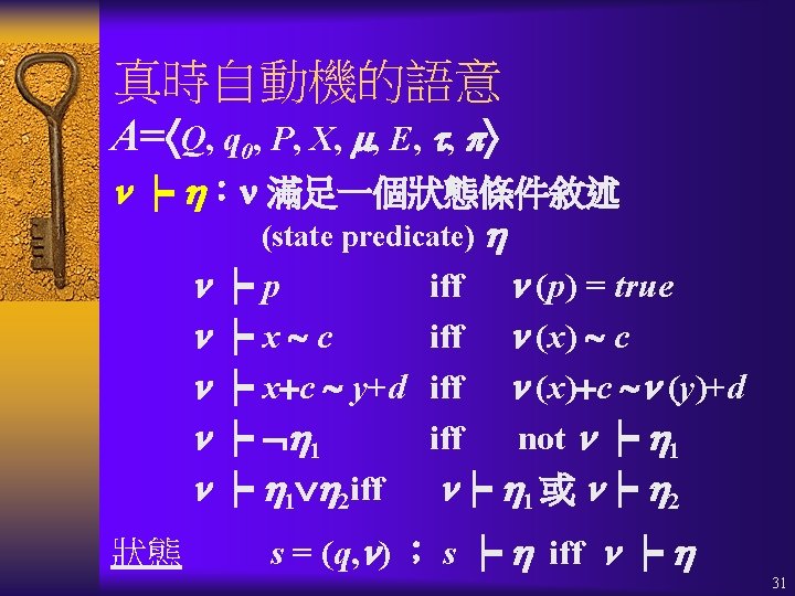
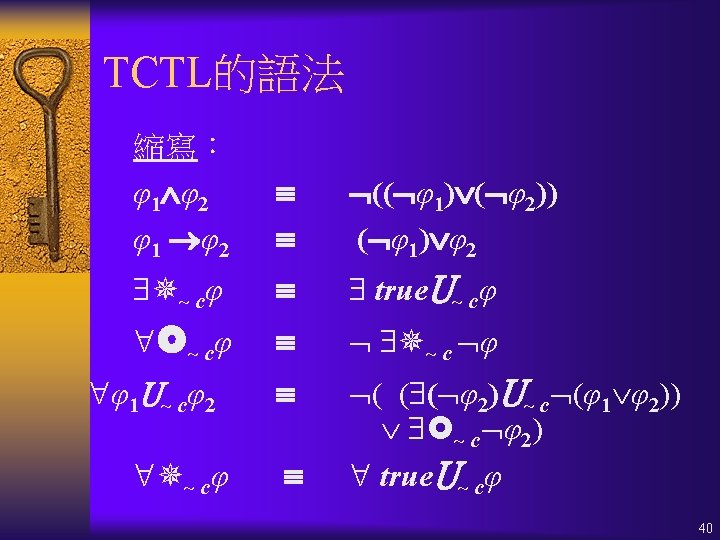
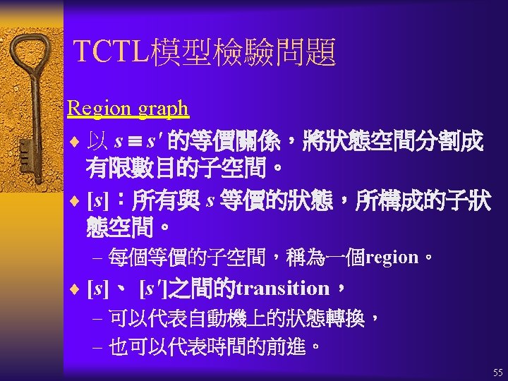
DBM (3 operations: Clock Reset) D' = D [Y : = 0], Y X defined as follows: ¨ Clock Reset: • D'(i, j) = ( 0) if xi, xj Y • D'(i, j) = D(0, j) Y if xi Y and xj • D'(i, j) = D(i, 0) Y if xj Y and xi • D'(i, j) = D(i, j)if xj Y and xi Y 70
DBM (3 operations: Time Elapse) ¨ Time Elapse: D' = te(D) defined as follows: ¨ D'(i, 0) = (< ), for any i 0 ¨ D'(i, j) = D(i, j), for i = 0 or j 0 71
DBM (3 operations) ¨ All 3 operations can be efficiently implemented ¨ DBM must be canonalized (using tightening) before any of the 3 operations (intersection, clock reset, and time elapse) ¨ After any of the 3 operations, a DBM might no longer be canonical! ¨ Last step: Reduce to canonical form!!! 72
DBM (Zone Graph Construction) ¨ Clock zones: represented by DBM ¨ Succesor clock zones succ(z, e): computed by the 3 operations: intersection, reset, and time elapse on DBM instead of on clock zones 73
DBM (Zone Graph Construction) ¨ Initial state: (s 0, Z 0), Z 0: x = 0 y = 0 Zone D 0 74
DBM (Zone Graph Construction) ¨ Invariant (s 0) is 0≤x 0≤y≤ 5 75
DBM (Zone Graph Construction) ¨ Step 1: Intersection D 0 with (s 0) gives D 0 ¨ Step 2: Let time elapse: te(D 0 (s 0) ) 76
DBM (Zone Graph Construction) ¨ Step 3: Intersect with (s 0) again 77
DBM (Zone Graph Construction) ¨ Trigger (a) = y 3 78
DBM (Zone Graph Construction) ¨ Step 4: Intersect with trigger (a) 79
DBM (Zone Graph Construction) ¨ Step 5: Reset clock y in DBM Z 1 = 3 ≤ x ≤ 5 3 ≤ x y ≤ 5 y = 0 80
DBM (Zone Graph Construction) ¨ Successor of (s 0, Z 0) is (s 1, Z 1) ¨ Repeat the same 5 steps: ¨ (s 0, 4 ≤ y ≤ 5 4 ≤ y x ≤ 5 x = 0) ¨ (s 1, 0 ≤ x ≤ 1 0 ≤ x y ≤ 1 y = 0) ¨ (s 0, 5 ≤ y ≤ 8 5 ≤ y x ≤ 8 x = 0) ¨ (s 1, x = 0 y = 0), which is contained in the 2 nd zone, thus no more new zones can be generated!!! No more change! Stop! Zone Graph! 81
Binary Decision Diagram (BDD) ¨ BDD: A canonical form representation for Boolean formulas. ¨ Motivation: – Too much space redundancy in traditional representations – BDD is more compact than truth tables, conjunctive normal form, disjunctive normal form, binary decision trees, etc. – BDD has a canonical form – BDD operations are efficient 82
BDD (Binary Decision Tree) 83
BDD (redundancy in BDT) ¨ Binary Decision Trees (BDT): – Same size as truth tables – Lots of redundancy: Out of 8 subtrees rooted at b 2 only 3 are distinct!!! – Merge isomorphic subtrees BDD ¨ BDD is a rooted, DAG with 2 types of vertices: terminal and nonterminal ¨ Each nonterminal v is labeled with var(v) and has two successors: low(v) and high(v) ¨ Each terminal vertex is labeled 0 or 1 84
BDD (Boolean Function) ¨ BDD B with root v determines Boolean function fv(x 1, …, xn) as follows: ¨ If v is a terminal vertex fv(x 1, …, xn) = value(v) {0, 1} ¨ If v is a nonterminal vertex with var(v) = xi: fv(x 1, …, xn) = ( xi flow(v)(x 1, …, xn) ) ( xi fhigh(v)(x 1, …, xn)) 85
BDD (Canonical Form) ¨ Canonical Form: Two boolean functions are logically equivalent iff they have isomorphic representations ¨ Why Canonical Form? Simplifies equivalence checking and satisfiability checking ¨ BDD Canonical Form: 1. Same variable order along all paths from root to terminal 2. No isomorphic subtrees or redundant vertices 86
BDD (Canonical Form) ¨ For requirement 1 (same variable order): – Total ordering < on all variables – If u has a nonterminal successor v, then var(u) < var(v) ¨ For requirement 2 (no redundancy): Apply 3 transformations repeatedly: – Remove duplicate terminals – Remove duplicate non-terminals – Remove redundant tests 87
BDD (Canonical Form) ¨ Remove duplicate terminals: Eliminate all but one terminal vertex with a given label and redirect hanging arcs. ¨ Remove duplicate non-terminals: If var(u) = var(v), low(u) = low(v), high(u) = high(v), then eliminate u or v. Redirect hanging arcs. ¨ Remove redundant tests: If low(v) = high(v), then eliminate v and redirect incoming arcs to low(v). 88
BDD (Canonical Form) ¨ Apply 3 transformations repeatedly in a bottom-up manner ¨ Time: O(|BDD|) ¨ Gives Ordered BDD (OBDD) ¨ Order: a 1 < b 1 < a 2 < b 2 ¨ OBDD for two-bit comparator example 89
Ordered BDD (OBDD) ¨ Since OBDDs are canonical, it is easy to: – check equivalence = check BDD isomorphism – check satisfiability = check BDD isomorphism with OBDD(0) ¨ Size of OBDD depends critically on VARIABLE ORDERING!!! ¨ 2 -bit comparator example: Change variable order to: a 1 < a 2 < b 1 < b 2 11 vertices instead of 8 for a 1 < b 1 < a 2 < b 2 90
OBDD (Variable Ordering) ¨ a 1 < a 2 < b 1 < b 2 ¨ In general, for n-bit comparator: a 1 < b 1 < …< an < bn gives 3 n + 2 vertices a 1 < …< an < b 1<…< bn gives 3 2 n 1 vertices 91
OBDD (Variable Ordering) ¨ Infeasible to find an optimal variable ordering! ¨ Checking a particular ordering is optimal is NP-complete! ¨ There are Boolean functions with exponential size OBBDs for any ordering! ¨ Eg: nth output of a combinational circuit to multiply two n bit integers 92
OBDD (Variable Ordering) ¨ Heuristics to find a good variable ordering: ¨ Depth-First Traversal of circuit gives a good variable order ¨ Intuition: related variables should be grouped together in the order ¨ Dynamic Reordering: – to save time and space, – not to find an optimal ordering. 93
OBDD (Operations) ¨ All 16 two-argument logical operations can be implemented efficiently on OBDDs. ¨ Time Complexity = O(|OBDD 1| |OBDD 2|) ¨ Key Idea: Shannon Expansion f = ( x f |x: =0) (x f |x: =1) ¨ Let f, f ' = OBDDs, v, v' = roots, x = var(v), x' = var(v') ¨ Apply(f, f ', *, ): a uniform algorithm for all 16 operations * 94
OBDD (Apply Algorithm) ¨ If v, v' are terminals, f * f ' = value(v) * value(v') ¨ If x = x', then use Shannon Expansion: f * f ' = ( x (f |x: =0 * f '|x: =0)) ( x f |x: =1 * f '|x: =1)) ¨ If x < x', then Shannon Expansion simplifies: f * f ' = ( x (f |x: =0* f ')) (x f |x: =1 * f ')) (∵ f '|x: =0 = f '|x: =1 = f ' does not depend on x) 95
OBDD (Efficiency) ¨ A problem generates 2 sub-problems ¨ Use dynamic programming to avoid exponential algorithm ¨ # sub-graphs = |OBDD(f )| ¨ A sub-problem depends on 2 sub-graphs ¨ # sub-problems ≤ |OBDD(f 1)| |OBDD(f 2)| ¨ Result Cache: computed sub-problems in canonical form ¨ Modern BDD package: millions of vertices! 96
OBDD (Representing Kripke Structures) ¨ State variables: a, b ¨ Add new state variables: a', b' ¨ s 1 s 2: (a b a' b') ¨ Full system: (a b a' b') 97
Symbolic Model Checking ¨ Symbolic = Manipulation of Boolean formulas ¨ Symbolic Operate on entire sets of states instead of individual states and transitions 98
Fixpoint Representations ¨ M(S, R, L): Finite Kripke Structure ¨ P(S): power set of S ¨ Least element in P(S): False = empty set ¨ Greatest element in P(S): True = S ¨ Predicate transformer: : P(S) ¨ 0(Z) = Z, i+1(Z) = i(Z) ¨ is monotonic if P Q (P) (Q) 99
Fixpoint Representations ¨ Fixpoint characterization of temporal logic operators ¨ A set S' S is a fixpoint of a function : P(S) if (S') = S'. (S: set of states, P(S): power set of S) ¨ A monotonic predicate transformer on P(S) always has: – a least fixpoint: Z. (Z) – a greatest fixpoint: Z. (Z) 100
Least Fixpoint ¨ False (False) 2(False) … ¨ No. of iterations |S| ¨ Last iteration: (Q) = Q = Z. (Z) (False) False 101
Least Fixpoint Algorithm 102
Greatest Fixpoint ¨ True (True) 2(True) … ¨ No. of iterations |S| ¨ Last iteration: (Q) = Q = Z. (Z) True = S (True) 2 (True) Z. (Z) 103
Greatest Fixpoint Algorithm 104
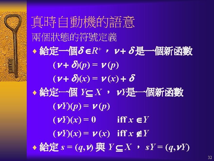
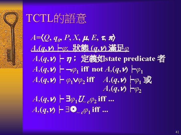
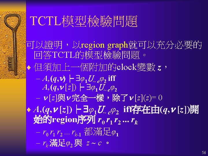
Fixpoint Characterizations ¨ = Z. Z ¨ = Z. Z ¨ [ 1 U 2] = Z. 2 ( 1 Z) Z Z 105
Approximations for [p U q] 106
Symbolic Model Checking for CTL ¨ Kripke Structures are represented symbolically using OBDDs. ¨ Quantified Boolean Formulas QBF(V): – every propositional variable in V is a formula – f, f g are formulas, if f and g are – v f and v f are formulas, if f is and v V ¨ Every QBF formula can be represented by an OBDD x f = f |x=0 f |x=1 107
Symbolic Model Checking Algorithm ¨ Check(a CTL formula) returns an OBDD that represents all system states satisfying the formula ¨ Inductive definition of Check() as follows: – If f = a (a proposition), Check(f ) returns the set of states satisfying a. – If f = f 1 f 2 or f = f 1, use Apply(Check(f 1), Check(f 2), *) 108
Symbolic Model Checking Algorithm ¨ Check( f ) = Check. EX(Check(f )) ¨ Check( [f U g]) = Check. EU(Check(f ), Check(g)) ¨ Check( f ) = Check. EG(Check(f )) CTL formula OBDD 109
Check. EX(f ) ¨ f is true in a state if it has a successor in which f is true. = v'[f (v') R(v, v')] = [f (v') R(v, v')]|v'=0 [f (v') R(v, v')]|v'=1 ¨ Check. EX(f (v)) ¨ R is the transition relation OBDD ¨ Given OBDDs for f and R, we can compute an OBDD for v'[f (v') R(v, v')] 110
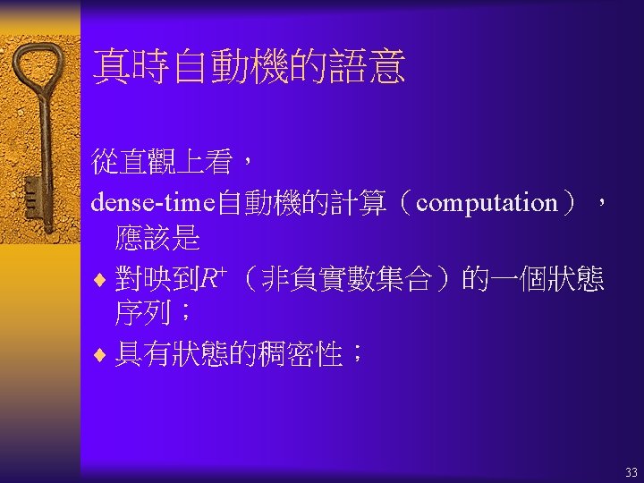
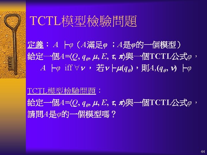
Check. EU(f ) ¨ Least fixpoint characterization: [ 1 U 2] = Z. 2 ( 1 Z) ¨ Use Lfp() to compute Q 0=False, Q 1, …, Qi, … that converges to [ 1 U 2] ¨ Given OBDDs for 1, 2, and Qi, we can compute Qi+1. ¨ Qi+1= 2 ( 1 Qi) ¨ Qi+1= Qi Qi= Z. 2 ( 1 Z) 111
Check. EG(f ) ¨ Greatest fixpoint characterization = Z. Z ¨ Use Gfp() to compute Q 0=True, Q 1, …, Qi, … that converges to ¨ Given OBDDs for 1 and Qi, we can compute Qi+1. ¨ Qi+1 = Qi ¨ Qi+1= Qi Qi= Z. Z 112
Fairness in Symbolic Model Checking ¨ Fairness Constraints F = {P 1, …, Pn} ¨ = Z. k = 1…n [ U(Z Pk)] ¨ Set of all states which are start of some fair computation is fair(v) = Check. Fair( True) ¨ Check. Fair. EX(f (v)) = Check. EX(f (v) fair(v)) ¨ Check. Fair. EU(f(v), g(v)) = Check. EU(f(v), g(v) fair(v)) 113
Counterexamples & Witnesses ¨ Counterexample: If is false, produce a path to a state in which holds. ¨ Witness: If is true, produce a path to a state in which holds. ¨ Counterexample( ) = Witness( ) ¨ Thus, need consider only witnesses: , U, and . 114
Witnesses ¨ Construct SCC graph G(V, E), where each node in V is an SCC, and an edge exists if there is a transition from a state in one SCC to a state in another SCC. ¨ SCC graph contains no cycle (because all cycles are in SCC graph nodes) ¨ Each infinite path has a suffix in an SCC graph node. 115
Witness for with F = {P 1, …, Pk} ¨ = Z. k = 1…n [ U(Z Pk)] ¨ For each P, compute an increasing sequence of approximations Q 0 P Q 1 P Q 2 P …, where Qi. P is the set of states from which a state in Z P can be reached in i steps. ¨ Start with an initial state s satisfying f. ¨ Look for a successor t of s in Q 0 P, P F. ¨ If no such t, keep looking in Q 1 P, Q 2 P, … ¨ If t Qi. P and i > 0, find a successor of t in Qi-1 P, and continue until i = 0, thus we have a path from s to some state u in P. Continue with other P F to obtain s'. Find a path from s' to t (cycle). 116
Witness for in first SCC 117
Witness for spans 3 SCC 118
Witnesses for U and ¨ fair = {s | state s satisfies True with F} ¨ Witness for [ f U g] with F = Witness for [ f U (g fair)] ¨ Witness for [ f ] with F = Witness for [ f fair] 119
An ALU Example 120
An ALU Example Pipeline circuit ¨ First cycle of instruction: read operands from register file into operand registers ¨ Second cycle: compute result and store in first pipe register ¨ Third to r + 1 cycle: result is passed through remaining pipeline registers ¨ Last cycle: result is written to register file 121
An ALU Example ¨ Only after r + 2 cycles, the result of an operation is written back to register file. ¨ Input signal stall invalid instruction (e. g. , cache miss) no change to destination reg ¨ Assume: 1 pipe register, XOR op only ¨ CTL specification has 2 parts: – Destination register updated correctly – All other registers should not change 122
An ALU Example Spec Part 1 (Dest reg updated correctly) ¨ Use n operator for n cycle delays ¨ src 1 opi = ( src 1 addr 2 reg 0, i) (src 1 addr 2 reg 1, i) ¨ src 2 opi = ( src 2 addr 2 reg 0, i) (src 2 addr 2 reg 1, i) ¨ resulti = ( destaddr 3 reg 0, i) (destaddr 3 reg 1, i) 123
An ALU Example Spec Part 2 (No change in other registers) ¨ ((stall destaddr) ( 2 reg 0, i 3 reg 0, i)) ¨ ((stall destaddr) ( 2 reg 1, i 3 reg 1, i)) 124
An ALU Example (Experiment Results) ¨ 8 -bit wide pipeline ¨ 4 general registers ¨ 1 pipeline register ¨ 1 operation ¨ More than 1020 states ¨ 41, 000 OBDD nodes ¨ Verification time: 22 mins of Sun 3 ¨ Substantial improvement over explicit-state model checking 125