Model Checking in the Proportional Hazard model Model
- Slides: 21

Model Checking in the Proportional Hazard model

• Model adequacy • Influential observations • PH assumption • Example: leaders data • Total 472 observations • Total 11 covariates fitted in the initial PH model • Manner start age conflict loginc region

Assessing model adequacy (1) Residuals checking: • • • Cox-Snell (& modified) Martingale Deviance Schoenfeld Score

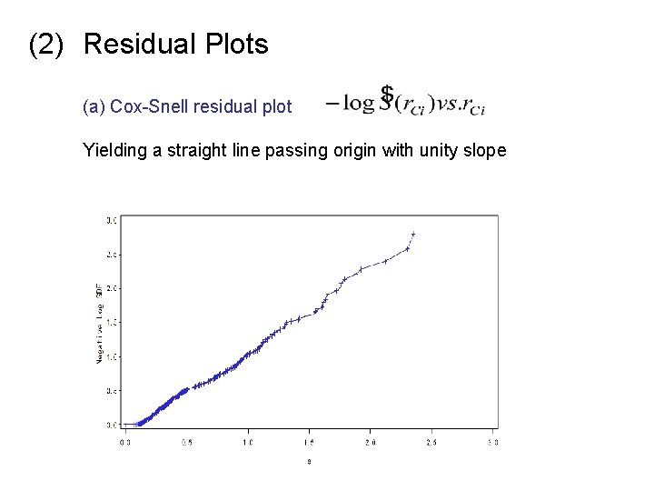
(2) Residual Plots (a) Cox-Snell residual plot Yielding a straight line passing origin with unity slope

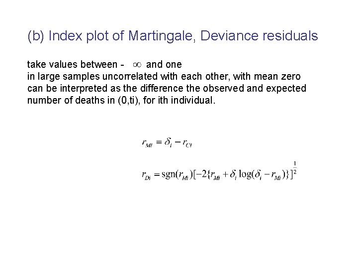
(b) Index plot of Martingale, Deviance residuals take values between and one in large samples uncorrelated with each other, with mean zero can be interpreted as the difference the observed and expected number of deaths in (0, ti), for ith individual.

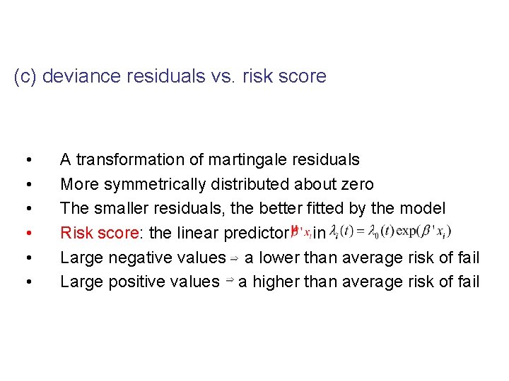
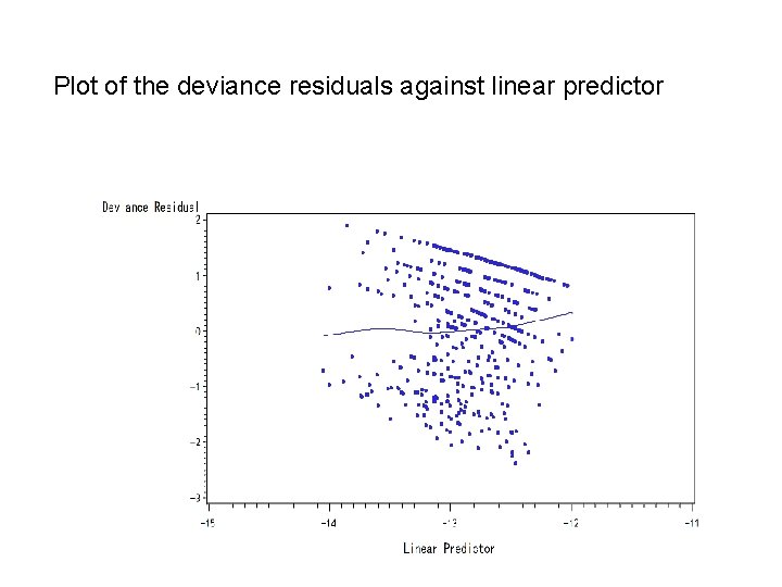
(c) deviance residuals vs. risk score • • • A transformation of martingale residuals More symmetrically distributed about zero The smaller residuals, the better fitted by the model Risk score: the linear predictor in Large negative values a lower than average risk of fail Large positive values a higher than average risk of fail

Plot of the deviance residuals against linear predictor

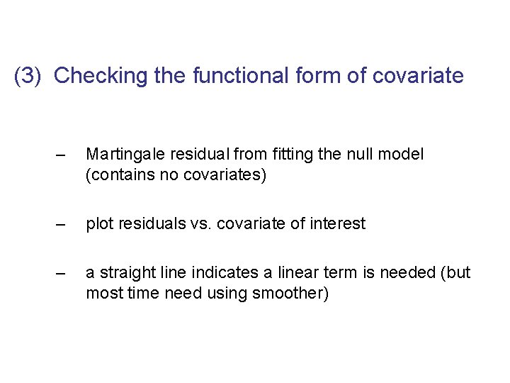
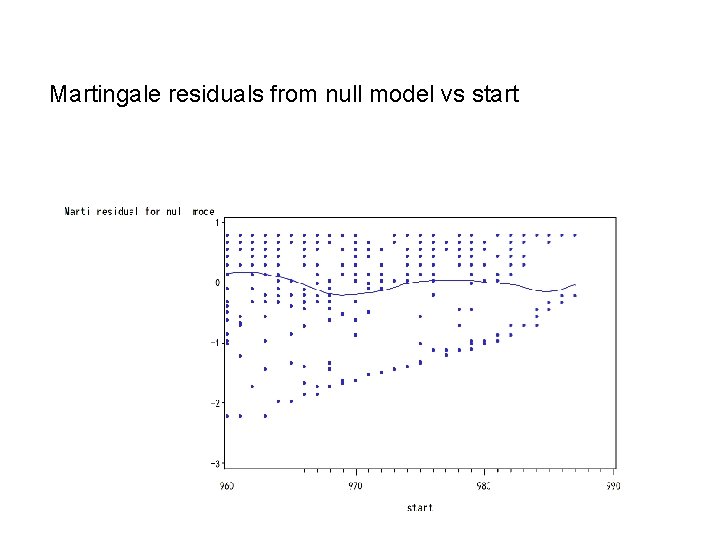
(3) Checking the functional form of covariate – Martingale residual from fitting the null model (contains no covariates) – plot residuals vs. covariate of interest – a straight line indicates a linear term is needed (but most time need using smoother)

Martingale residuals from null model vs start

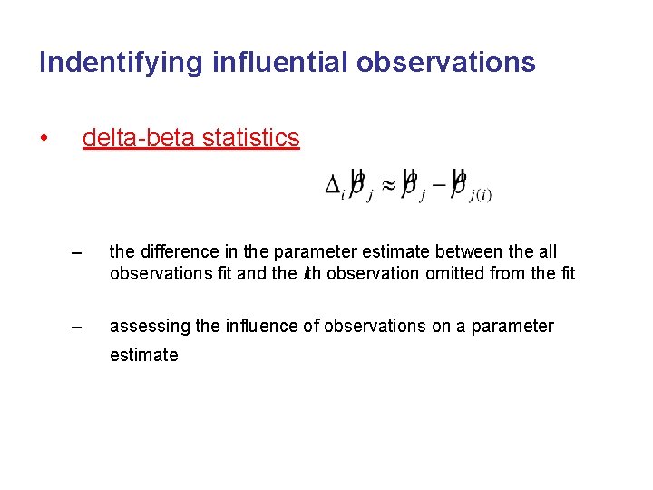
Indentifying influential observations • delta-beta statistics – the difference in the parameter estimate between the all observations fit and the ith observation omitted from the fit – assessing the influence of observations on a parameter estimate

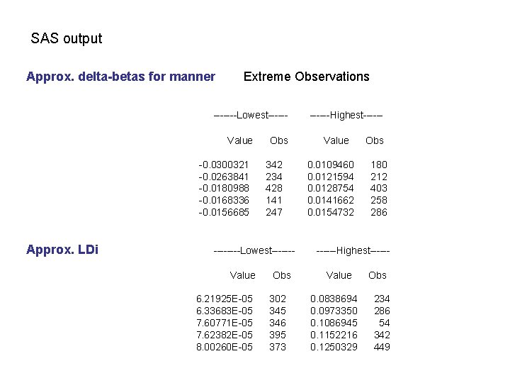
SAS output Approx. delta-betas for manner Extreme Observations -------Lowest-----Value -0. 0300321 -0. 0263841 -0. 0180988 -0. 0168336 -0. 0156685 Approx. LDi Obs 342 234 428 141 247 ----Lowest------Value 6. 21925 E-05 6. 33683 E-05 7. 60771 E-05 7. 62382 E-05 8. 00260 E-05 Obs 302 345 346 395 373 ------Highest-----Value 0. 0109460 0. 0121594 0. 0128754 0. 0141662 0. 0154732 Obs 180 212 403 258 286 ------Highest-----Value 0. 0838694 0. 0973350 0. 1086945 0. 1152216 0. 1250329 Obs 234 286 54 342 449

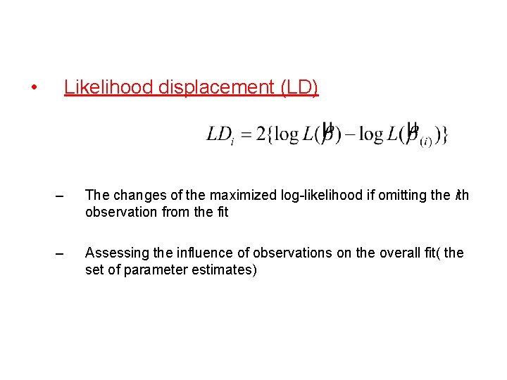
• Likelihood displacement (LD) – The changes of the maximized log-likelihood if omitting the ith observation from the fit – Assessing the influence of observations on the overall fit( the set of parameter estimates)

• Treatment: – Check the original data, corrected it if found any mistakes – Make inferences based on both situations (full & reduced data), contrast results

Testing PH assumption • A crucial assumption when using Cox model • The effect of covariates on the hazard rate are the same over time

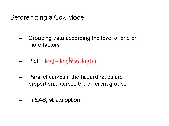
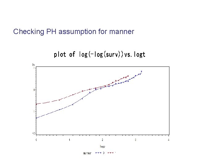
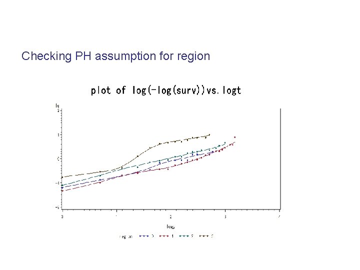
Before fitting a Cox Model – Grouping data according the level of one or more factors – Plot – Parallel curves if the hazard ratios are proportional across the different groups – In SAS, strata option

Checking PH assumption for manner

Checking PH assumption for region

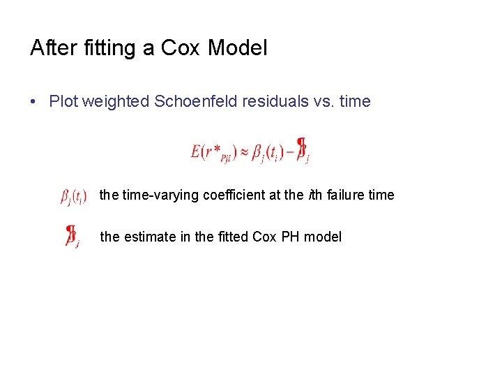
After fitting a Cox Model • Plot weighted Schoenfeld residuals vs. time the time-varying coefficient at the ith failure time the estimate in the fitted Cox PH model

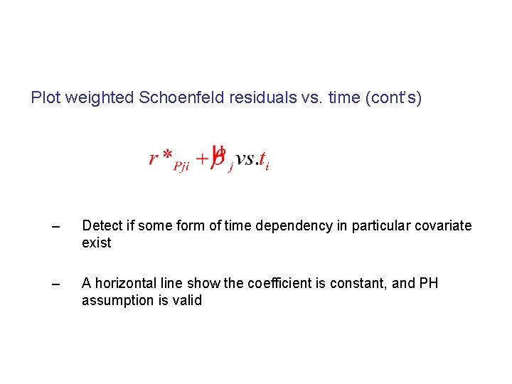
Plot weighted Schoenfeld residuals vs. time (cont’s) – Detect if some form of time dependency in particular covariate exist – A horizontal line show the coefficient is constant, and PH assumption is valid

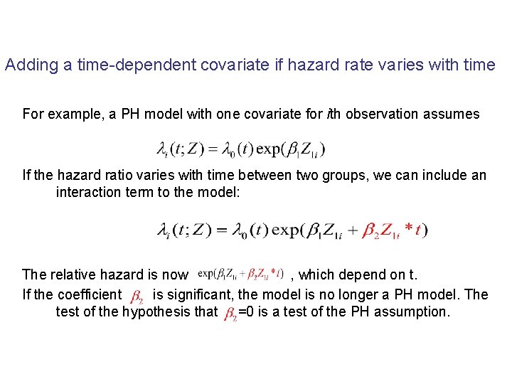
Adding a time-dependent covariate if hazard rate varies with time For example, a PH model with one covariate for ith observation assumes If the hazard ratio varies with time between two groups, we can include an interaction term to the model: The relative hazard is now , which depend on t. If the coefficient is significant, the model is no longer a PH model. The test of the hypothesis that =0 is a test of the PH assumption.

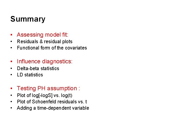
Summary • Assessing model fit: • Residuals & residual plots • Functional form of the covariates • Influence diagnostics: • Delta-beta statistics • LD statistics • Testing PH assumption : • Plot of log[-log. S] vs. log(t) • Plot of Schoenfeld residuals vs. t • Adding a time-dependent variable