Propensity Scores Friday June 1 st 10 15

Propensity Scores Friday, June 1 st, 10: 15 am-12: 00 pm Deborah Rosenberg, Ph. D Kristin Rankin, Ph. D Research Associate Professor Research Assistant Professor Division of Epidemiology and Biostatistics University of IL School of Public Health Training Course in MCH Epidemiology

Propensity Scores The goal of using propensity scores is to more completely and efficiently address observed confounding of an exposureoutcome relationship. Program evaluation – Addresses selection bias Epidemiology – Addresses non-randomization of exposure Propensity scores are the predicted probabilities from a regression model of this form: Exposure = pool of observed confounders “Conditional probability of being exposed or treated (or both)” 1

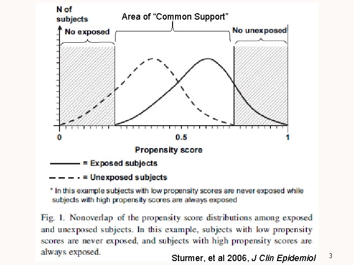
Propensity Scores When exposed and unexposed groups are not equivalent such that the distribution on covariates is not only different, but includes non-overlapping sets of values, then the usual methods for controlling for confounding may be inadequate. Non-overlapping distributions (lack of common support) means that individuals in one group have values on some of the covariates that don’t exist in the other group and vice versa. 2

Area of “Common Support” Sturmer, et al 2006, J Clin Epidemiol 3

Benefits of Propensity Score Methods The accessibility of multivariable regression methods means they are often misused, with reporting of estimates that are extrapolations beyond available data. The process of generating propensity scores: – focuses attention on model specification to account for covariate imbalance across exposure groups, and support of data with regard to “exchangeability” of exposed and unexposed – Allows for trying to mimic randomization by simultaneously matching people on large sets of known covariates – Forces researcher to design study/check covariate balance before looking at outcomes Oakes and Johnson, Methods in Social Epidemiology 4

Propensity Scores Propensity scores might be used in three ways: 1. as a covariate in a model along with exposure, or as weights for the observations in a crude model (not recommended due to possible off-support inference) 2. as values on which to stratify/subclassify data to form more comparable groups 3. as values on which to match an exposed to an unexposed observation, then using the matched pair in an analysis that accounts for the matching 5

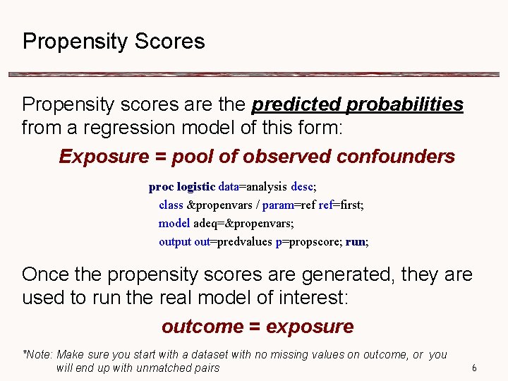
Propensity Scores Propensity scores are the predicted probabilities from a regression model of this form: Exposure = pool of observed confounders proc logistic data=analysis desc; class &propenvars / param=ref ref=first; model adeq=&propenvars; output out=predvalues p=propscore; run; Once the propensity scores are generated, they are used to run the real model of interest: outcome = exposure *Note: Make sure you start with a dataset with no missing values on outcome, or you will end up with unmatched pairs 6

Generating Propensity Scores • Consider only covariates that are measured preprogram/intervention/exposure or do not change over time; value shouldn’t be affected by exposure or in causal pathway between exposure and outcome • Covariates should be based on theory or prior empirical findings; never use model selection procedures such as stepwise selection for these covariates – if conceptually based, they should stay in the model regardless of statistical significance • Include higher order terms and interactions to get best estimated probability of exposure and balance across covariates; trade-off between fully accounting for confounding and including so many unnecessary variables/terms that common support becomes an issue and PS distributions are more likely to be non-overlapping Oakes and Johnson, Methods in Social Epidemiology 7

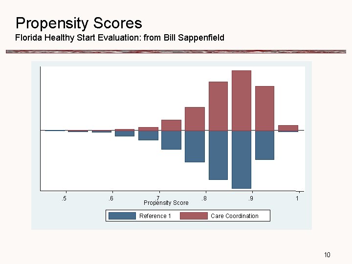
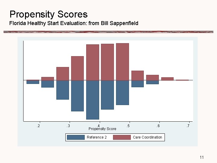
Propensity Score Distributions Examine the distribution of propensity scores in exposed and unexposed • If there is not enough overlap (not enough “common support”), then these data cannot be used to answer the research question • Observations with no overlap cannot be used in matched analysis • If there areas that don’t overlap, the matched sample may not be representative (examine characteristics of excluded individuals to assess this) 8

Propensity Scores • Sometimes propensity scores are used to verify that pre-defined comparison groups are actually equivalent; • If they are, then the propensity scores may not have to be used in analysis 9

Propensity Scores Florida Healthy Start Evaluation: from Bill Sappenfield . 5 . 6 . 7 Propensity Score Reference 1 . 8 . 9 1 Care Coordination 10

Propensity Scores Florida Healthy Start Evaluation: from Bill Sappenfield . 2 . 3 . 4 Propensity Score Reference 2 . 5 . 6 . 7 Care Coordination 11

Analysis Approach 1: Propensity Score as a Covariate or Weight in Model • Use the propensity score as a covariate in model – 1 degree of freedom as opposed to 1 or more for each original covariate; particularly useful when the prevalence of outcome is small relative to the number of covariates that must be controlled, leading to small cell sizes • Weight data using the propensity scores –the weight for an “exposed” subject is the inverse of the propensity score –the weight for an “unexposed” subject is the inverse of 1 minus propensity score; weights must be normalized These approaches do not handle the issue of off-support data unless data are restricted to the range of propensity scores common to both the exposed and unexposed 12

Analysis Approach 2: Subclassification by Categories of the Propensity Scores § Stratifying by quintiles of the overall distribution of propensity scores can remove approx 90% of the bias caused by the propensity score § The measure of effect is then computed in each stratum and a weighted average is estimated based on the number of observations in each stratum 13

Analysis Approach 3: Propensity Score Matching Several matching techniques are available: • Nearest Neighbor (with or without replacement) • Caliper and Radius • Kernal and Local Linear Several software solutions available to perform matching. Two examples include: • PSMATCH 2 in STATA • GREEDY macro in SAS 14

Analysis Approach 3: Propensity Score Matching PSMATCH 2 (STATA): • PSMATCH 2 is flexible and user-controlled with regard to matching techniques GREEDY (5 1 digit) macro in SAS: • The GREEDY (5 1 digit) Macro in SAS performs one to one nearest neighbor within-caliper matching: • First, matches are made within a caliper width of 0. 00001 (“best matches”), then caliper width decreases incrementally for unmatched cases to 0. 1 • At each stage, “unexposed” subject with “closest” ; propensity score is selected as the match to the exposed; in the case of ties, the unexposed is randomly selected • Sampling is without replacement 15

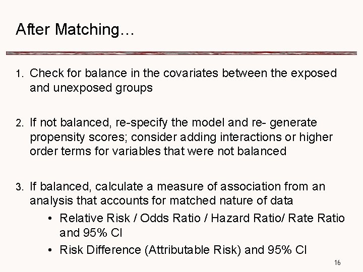
After Matching… 1. Check for balance in the covariates between the exposed and unexposed groups 2. If not balanced, re-specify the model and re- generate propensity scores; consider adding interactions or higher order terms for variables that were not balanced 3. If balanced, calculate a measure of association from an analysis that accounts for matched nature of data • Relative Risk / Odds Ratio / Hazard Ratio/ Rate Ratio and 95% CI • Risk Difference (Attributable Risk) and 95% CI 16

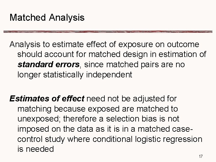
Matched Analysis to estimate effect of exposure on outcome should account for matched design in estimation of standard errors, since matched pairs are no longer statistically independent Estimates of effect need not be adjusted for matching because exposed are matched to unexposed; therefore a selection bias is not imposed on the data as it is in a matched case- control study where conditional logistic regression is needed 17

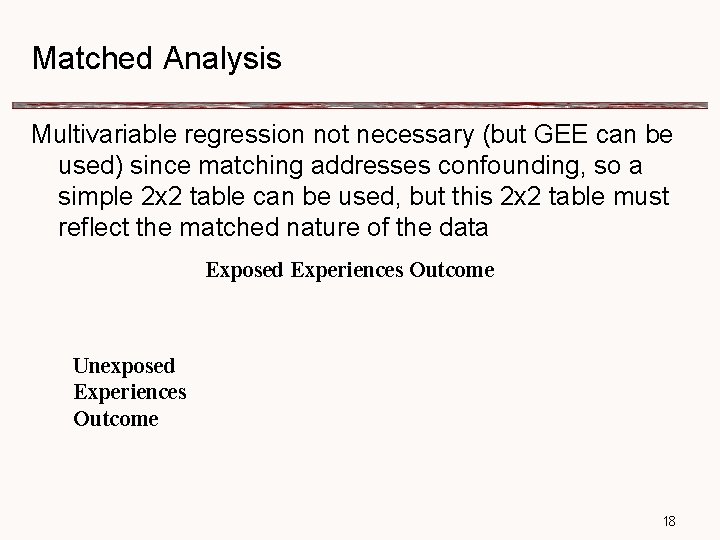
Matched Analysis Multivariable regression not necessary (but GEE can be used) since matching addresses confounding, so a simple 2 x 2 table can be used, but this 2 x 2 table must reflect the matched nature of the data Exposed Experiences Outcome Unexposed Experiences Outcome 18

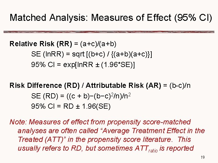
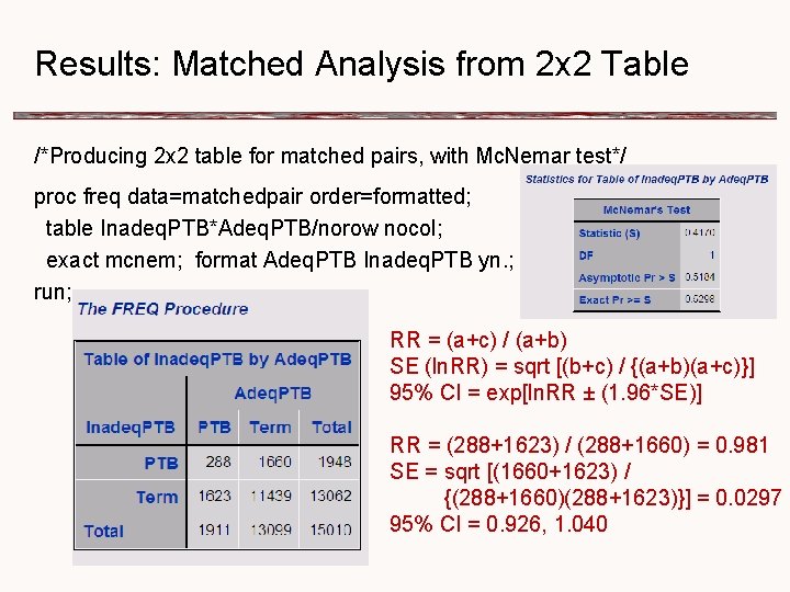
Matched Analysis: Measures of Effect (95% CI) Relative Risk (RR) = (a+c)/(a+b) SE (ln. RR) = sqrt [(b+c) / {(a+b)(a+c)}] 95% CI = exp[ln. RR ± (1. 96*SE)] Risk Difference (RD) / Attributable Risk (AR) = (b-c)/n SE (RD) = ((c + b)−(b−c)2/n)/n 2 95% CI = RD ± 1. 96(SE) Note: Measures of effect from propensity score-matched analyses are often called “Average Treatment Effect in the Treated (ATT)” in the propensity score literature. This usually refers to RD, but sometimes ATTratio is reported 19

Propensity Scores Using the 2007 National Survey of Children’s Health (NSCH) for Illinois 20

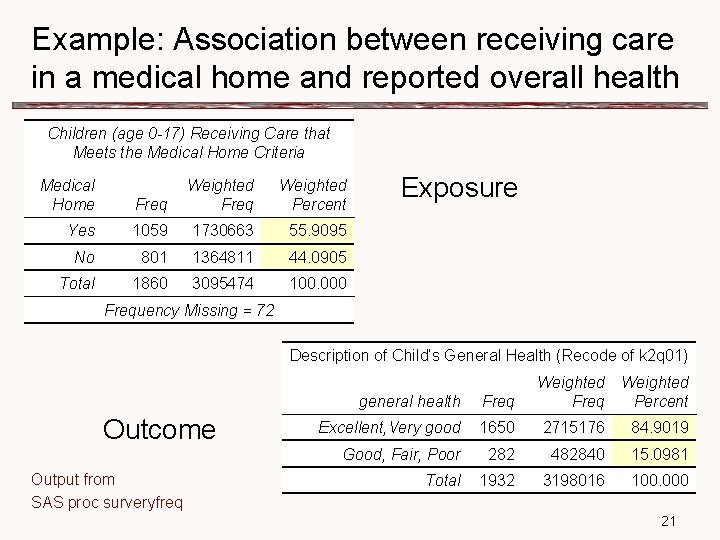
Example: Association between receiving care in a medical home and reported overall health Children (age 0 -17) Receiving Care that Meets the Medical Home Criteria Medical Home Freq Weighted Percent Yes 1059 1730663 55. 9095 No 801 1364811 44. 0905 Total 1860 3095474 100. 000 Exposure Frequency Missing = 72 Description of Child’s General Health (Recode of k 2 q 01) Outcome Output from SAS proc surveryfreq general health Freq Weighted Percent Excellent, Very good 1650 2715176 84. 9019 Good, Fair, Poor 282 482840 15. 0981 Total 1932 3198016 100. 000 21

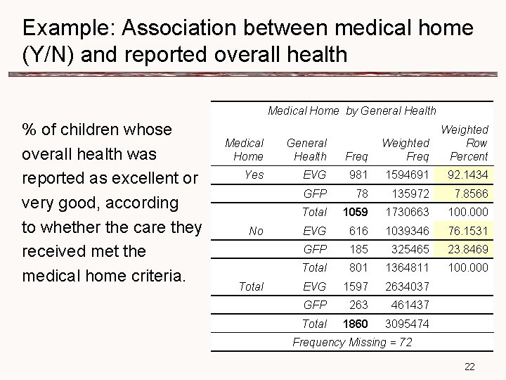
Example: Association between medical home (Y/N) and reported overall health Medical Home by General Health % of children whose overall health was reported as excellent or very good, according to whether the care they received met the medical home criteria. Freq Weighted Row Percent EVG 981 1594691 92. 1434 GFP 78 135972 7. 8566 Total 1059 1730663 100. 000 EVG 616 1039346 76. 1531 GFP 185 325465 23. 8469 Total 801 1364811 100. 000 EVG 1597 2634037 GFP 263 461437 Total 1860 3095474 Medical Home General Health Yes No Total Frequency Missing = 72 22

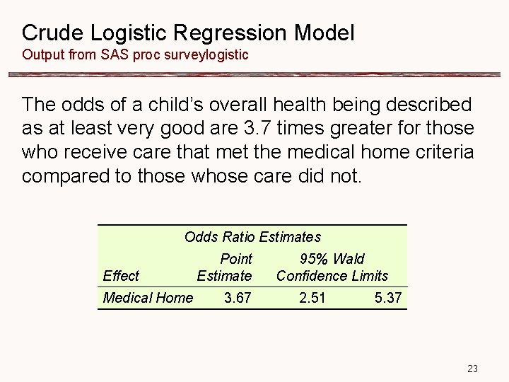
Crude Logistic Regression Model Output from SAS proc surveylogistic The odds of a child’s overall health being described as at least very good are 3. 7 times greater for those who receive care that met the medical home criteria compared to those whose care did not. Odds Ratio Estimates Effect Medical Home Point Estimate 3. 67 95% Wald Confidence Limits 2. 51 5. 37 23

Creating Propensity Scores for the Medical Home § Many factors—sociodemographic as well as medical—are likely to confound the association between medical home and reported overall health. § It may not be feasible to adjust for all of these factors in a conventional regression model. § Instead, propensity scores will be generated to simultaneously account for many factors. 24

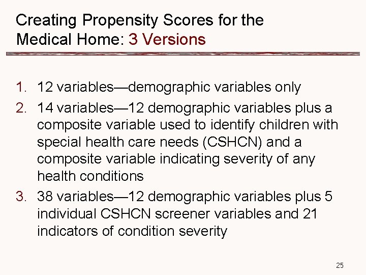
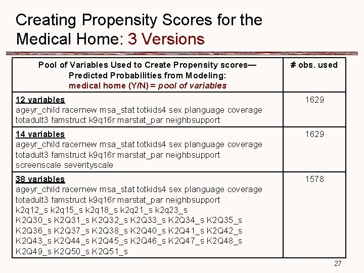
Creating Propensity Scores for the Medical Home: 3 Versions 1. 12 variables—demographic variables only 2. 14 variables— 12 demographic variables plus a composite variable used to identify children with special health care needs (CSHCN) and a composite variable indicating severity of any health conditions 3. 38 variables— 12 demographic variables plus 5 individual CSHCN screener variables and 21 indicators of condition severity 25

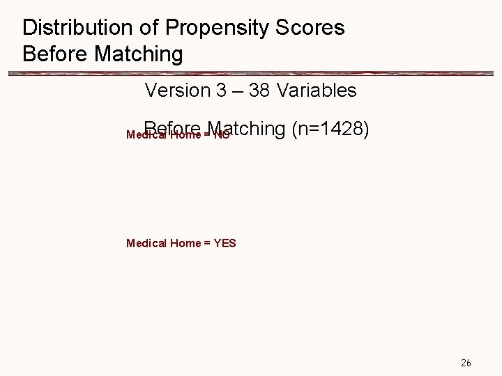
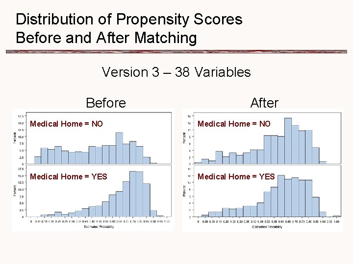
Distribution of Propensity Scores Before Matching Version 3 – 38 Variables Before Matching (n=1428) Medical Home = NO Medical Home = YES 26

Creating Propensity Scores for the Medical Home: 3 Versions Pool of Variables Used to Create Propensity scores— Predicted Probabilities from Modeling: medical home (Y/N) = pool of variables # obs. used 12 variables ageyr_child racernew msa_stat totkids 4 sex planguage coverage totadult 3 famstruct k 9 q 16 r marstat_par neighbsupport 1629 14 variables ageyr_child racernew msa_stat totkids 4 sex planguage coverage totadult 3 famstruct k 9 q 16 r marstat_par neighbsupport screenscale severityscale 1629 38 variables ageyr_child racernew msa_stat totkids 4 sex planguage coverage totadult 3 famstruct k 9 q 16 r marstat_par neighbsupport k 2 q 12_s k 2 q 15_s k 2 q 18_s k 2 q 21_s k 2 q 23_s K 2 Q 30_s K 2 Q 31_s K 2 Q 32_s K 2 Q 33_s K 2 Q 34_s K 2 Q 35_s K 2 Q 36_s K 2 Q 37_s K 2 Q 38_s K 2 Q 40_s K 2 Q 41_s K 2 Q 42_s K 2 Q 43_s K 2 Q 44_s K 2 Q 45_s K 2 Q 46_s K 2 Q 47_s K 2 Q 48_s K 2 Q 49_s K 2 Q 50_s K 2 Q 51_s 1578 27

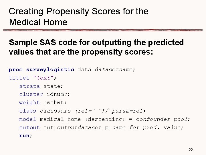
Creating Propensity Scores for the Medical Home Sample SAS code for outputting the predicted values that are the propensity scores: proc surveylogistic data=datasetname; title 1 “text”; strata state; cluster idnumr; weight nschwt; classvars (ref=“ “)/ param=ref; model medical_home (descending) = confounder pool; output out=outputdataset p=name for pred. value; run; 28

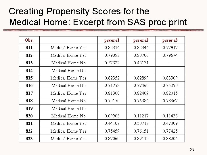
Creating Propensity Scores for the Medical Home: Excerpt from SAS proc print Obs. pscore 1 pscore 2 pscore 3 811 Medical Home Yes 0. 82314 0. 82344 0. 77917 812 Medical Home Yes 0. 79093 0. 80706 0. 79674 813 Medical Home No 0. 57322 0. 45131 . 814 Medical Home No . . . 815 Medical Home Yes 0. 82352 0. 82899 0. 83309 816 Medical Home No 0. 31732 0. 37460 0. 36290 817 Medical Home Yes 0. 81300 0. 82409 0. 82015 818 Medical Home No 0. 72170 0. 76384 0. 78867 819 Medical Home No . . . 820 Medical Home No 0. 09905 0. 11217 0. 11435 821 Medical Home Yes 0. 44107 0. 50713 0. 47309 822 Medical Home Yes 0. 75459 0. 76151 0. 77425 823 Medical Home Yes 0. 87060 0. 89112 0. 88204 29

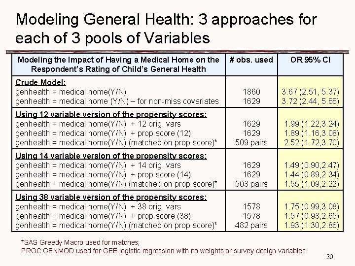
Modeling General Health: 3 approaches for each of 3 pools of Variables Modeling the Impact of Having a Medical Home on the Respondent’s Rating of Child’s General Health # obs. used OR 95% CI Crude Model: genhealth = medical home(Y/N) genhealth = medical home (Y/N) – for non-miss covariates 1860 1629 3. 67 (2. 51, 5. 37) 3. 72 (2. 44, 5. 66) Using 12 variable version of the propensity scores: genhealth = medical home(Y/N) + 12 orig. vars genhealth = medical home(Y/N) + prop score (12) genhealth = medical home(Y/N) (matched on prop score)* 1629 509 pairs 1. 99 (1. 22, 3. 24) 1. 89 (1. 16, 3. 08) 2. 52 (1. 72, 3. 70) Using 14 variable version of the propensity scores: genhealth = medical home(Y/N) + 14 orig. vars genhealth = medical home(Y/N) + prop score (14) genhealth = medical home(Y/N) (matched on prop score)* 1629 503 pairs 1. 49 (0. 90, 2. 47) 1. 44 (0. 89, 2. 34) 1. 55 (1. 09, 2. 22) Using 38 variable version of the propensity scores: genhealth = medical home(Y/N) + 38 orig. vars genhealth = medical home(Y/N) + prop score (38) genhealth = medical home(Y/N) (matched on prop score)* 1578 482 pairs 1. 75 (0. 99, 3. 08) 1. 57 (0. 93, 2. 65) 1. 93 (1. 30, 2. 86) *SAS Greedy Macro used for matches; PROC GENMOD used for GEE logistic regression with no weights or survey design variables. 30

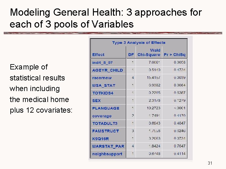
Modeling General Health: 3 approaches for each of 3 pools of Variables Example of statistical results when including the medical home plus 12 covariates: 31

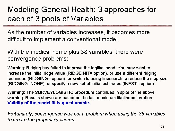
Modeling General Health: 3 approaches for each of 3 pools of Variables As the number of variables increases, it becomes more difficult to implement a conventional model. With the medical home plus 38 variables, there were convergence problems: Warning: Ridging has failed to improve the loglikelihood. You may want to increase the initial ridge value (RIDGEINIT= option), or use a different ridging technique (RIDGING= option), or switch to using linesearch to reduce the step size (RIDGING=NONE), or specify a new set of initial estimates (INEST= option). Warning: The SURVEYLOGISTIC procedure continues in spite of the above warning. Results shown are based on the last maximum likelihood iteration. Validity of the model fit is questionable. Fortunately, convergence was not a problem when using the 38 variables to create the propensity scores. 32

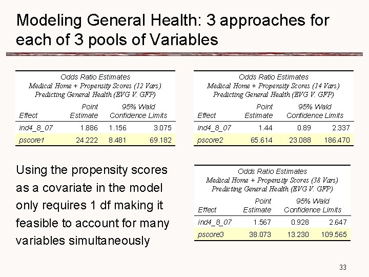
Modeling General Health: 3 approaches for each of 3 pools of Variables Odds Ratio Estimates Medical Home + Propensity Scores (12 Vars) Predicting General Health (EVG V. GFP) Effect ind 4_8_07 pscore 1 Point Estimate Odds Ratio Estimates Medical Home + Propensity Scores (14 Vars) Predicting General Health (EVG V. GFP) 95% Wald Confidence Limits Effect 1. 886 1. 156 3. 075 ind 4_8_07 24. 222 8. 481 69. 182 Using the propensity scores as a covariate in the model only requires 1 df making it feasible to account for many variables simultaneously pscore 2 Point Estimate 95% Wald Confidence Limits 1. 44 0. 89 2. 337 65. 614 23. 088 186. 470 Odds Ratio Estimates Medical Home + Propensity Scores (38 Vars) Predicting General Health (EVG V. GFP) Effect ind 4_8_07 pscore 3 Point Estimate 95% Wald Confidence Limits 1. 567 0. 928 2. 647 38. 073 13. 230 109. 565 33

Distribution of Propensity Scores Before and After Matching Version 3 – 38 Variables Before After Medical Home = NO Medical Home = YES

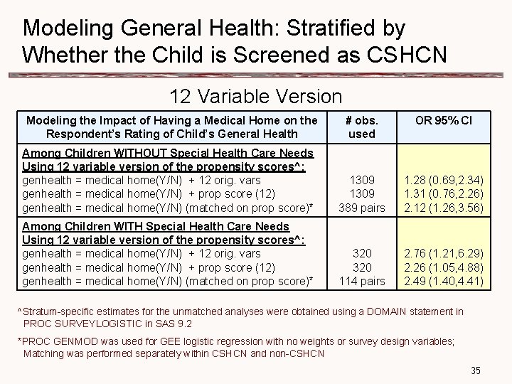
Modeling General Health: Stratified by Whether the Child is Screened as CSHCN 12 Variable Version Modeling the Impact of Having a Medical Home on the Respondent’s Rating of Child’s General Health # obs. used OR 95% CI Among Children WITHOUT Special Health Care Needs Using 12 variable version of the propensity scores^: genhealth = medical home(Y/N) + 12 orig. vars genhealth = medical home(Y/N) + prop score (12) genhealth = medical home(Y/N) (matched on prop score)* 1309 389 pairs 1. 28 (0. 69, 2. 34) 1. 31 (0. 76, 2. 26) 2. 12 (1. 26, 3. 56) Among Children WITH Special Health Care Needs Using 12 variable version of the propensity scores^: genhealth = medical home(Y/N) + 12 orig. vars genhealth = medical home(Y/N) + prop score (12) genhealth = medical home(Y/N) (matched on prop score)* 320 114 pairs 2. 76 (1. 21, 6. 29) 2. 26 (1. 05, 4. 88) 2. 49 (1. 40, 4. 41) ^Stratum-specific estimates for the unmatched analyses were obtained using a DOMAIN statement in PROC SURVEYLOGISTIC in SAS 9. 2 *PROC GENMOD was used for GEE logistic regression with no weights or survey design variables; Matching was performed separately within CSHCN and non-CSHCN 35

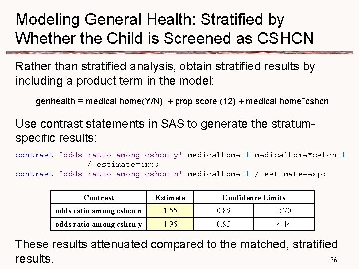
Modeling General Health: Stratified by Whether the Child is Screened as CSHCN Rather than stratified analysis, obtain stratified results by including a product term in the model: genhealth = medical home(Y/N) + prop score (12) + medical home*cshcn Use contrast statements in SAS to generate the stratumspecific results: contrast 'odds ratio among cshcn y' medicalhome 1 medicalhome*cshcn 1 / estimate=exp; contrast 'odds ratio among cshcn n' medicalhome 1 / estimate=exp; Contrast Estimate Confidence Limits odds ratio among cshcn n 1. 55 0. 89 2. 70 odds ratio among cshcn y 1. 96 0. 93 4. 14 These results attenuated compared to the matched, stratified 36 results.

Propensity Score Example: Using 2003 Natality Data for Illinois

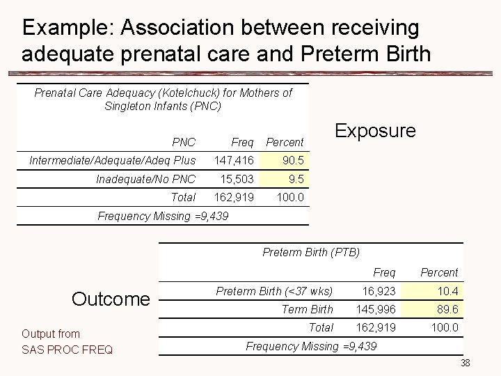
Example: Association between receiving adequate prenatal care and Preterm Birth Prenatal Care Adequacy (Kotelchuck) for Mothers of Singleton Infants (PNC) PNC Freq Percent Intermediate/Adequate/Adeq Plus 147, 416 90. 5 Inadequate/No PNC 15, 503 9. 5 Total 162, 919 100. 0 Exposure Frequency Missing =9, 439 Preterm Birth (PTB) Outcome Output from SAS PROC FREQ Freq Percent Preterm Birth (<37 wks) 16, 923 10. 4 Term Birth 145, 996 89. 6 Total 162, 919 100. 0 Frequency Missing =9, 439 38

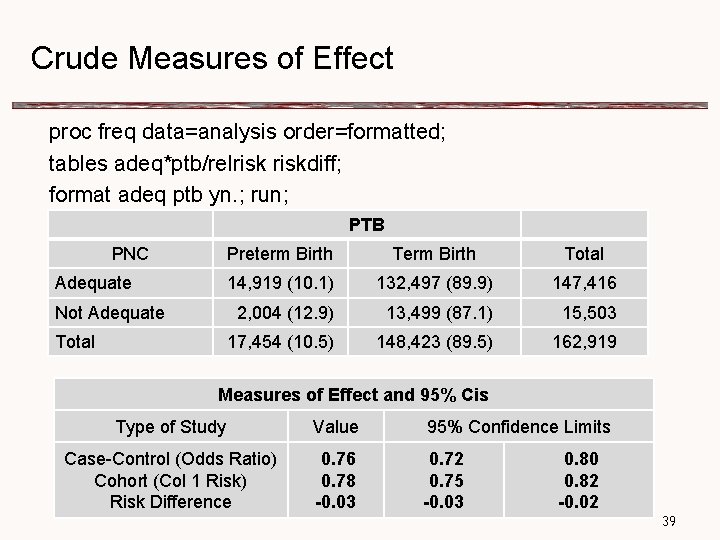
Crude Measures of Effect proc freq data=analysis order=formatted; tables adeq*ptb/relriskdiff; format adeq ptb yn. ; run; PTB PNC Preterm Birth Total Adequate 14, 919 (10. 1) 132, 497 (89. 9) 147, 416 Not Adequate 2, 004 (12. 9) 13, 499 (87. 1) 15, 503 Total 17, 454 (10. 5) 148, 423 (89. 5) 162, 919 Measures of Effect and 95% Cis Type of Study Value 95% Confidence Limits Case-Control (Odds Ratio) Cohort (Col 1 Risk) Risk Difference 0. 76 0. 78 -0. 03 0. 72 0. 75 -0. 03 0. 80 0. 82 -0. 02 39

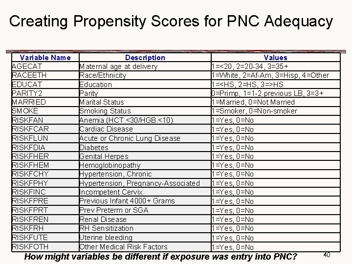
Creating Propensity Scores for PNC Adequacy Variable Name AGECAT RACEETH EDUCAT PARITY 2 MARRIED SMOKE RISKFAN RISKFCAR RISKFLUN RISKFDIA RISKFHER RISKFHEM RISKFCHY RISKFPHY RISKFINC RISKFPRE RISKFPRT RISKFREN RISKFRH RISKFUTE RISKFOTH Description Maternal age at delivery Race/Ethnicity Education Parity Marital Status Smoking Status Anemia (HCT. <30/HGB. <10) Cardiac Disease Acute or Chronic Lung Disease Diabetes Genital Herpes Hemoglobinopathy Hypertension, Chronic Hypertension, Pregnancy-Associated Incompetent Cervix Previous Infant 4000+ Grams Prev Preterm or SGA Renal Disease RH Sensitization Uterine bleeding Other Medical Risk Factors Values 1=<20, 2=20 -34, 3=35+ 1=White, 2=Af-Am, 3=Hisp, 4=Other 1=<HS, 2=HS, 3=>HS 0=Primp, 1=1 -2 previous LB, 3=3+ 1=Married, 0=Not Married 1=Smoker, 0=Non-smoker 1=Yes, 0=No 1=Yes, 0=No 1=Yes, 0=No 1=Yes, 0=No How might variables be different if exposure was entry into PNC? 40

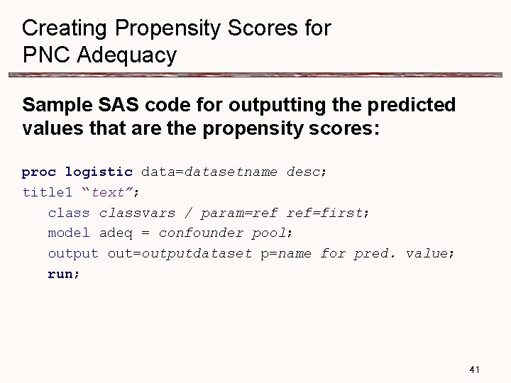
Creating Propensity Scores for PNC Adequacy Sample SAS code for outputting the predicted values that are the propensity scores: proc logistic data=datasetname desc; title 1 “text”; classvars / param=ref ref=first; model adeq = confounder pool; output out=outputdataset p=name for pred. value; run; 41

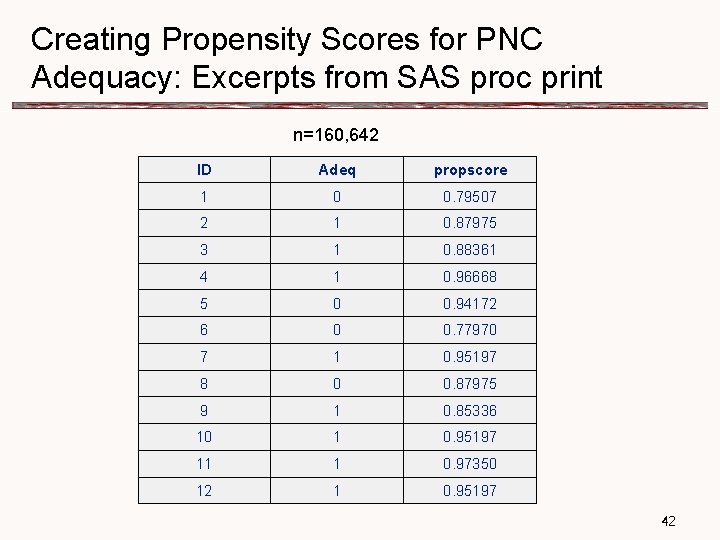
Creating Propensity Scores for PNC Adequacy: Excerpts from SAS proc print n=160, 642 ID Adeq propscore 1 0 0. 79507 2 1 0. 87975 3 1 0. 88361 4 1 0. 96668 5 0 0. 94172 6 0 0. 77970 7 1 0. 95197 8 0 0. 87975 9 1 0. 85336 10 1 0. 95197 11 1 0. 97350 12 1 0. 95197 42

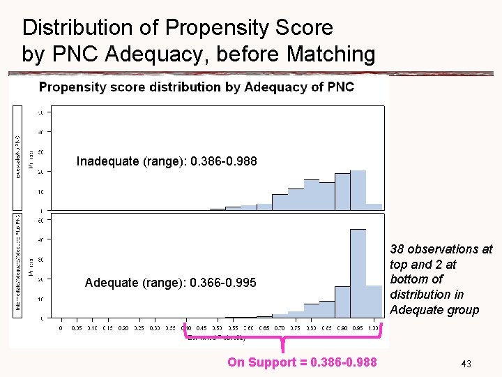
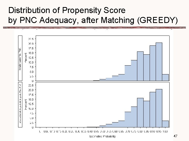
Distribution of Propensity Score by PNC Adequacy, before Matching Inadequate (range): 0. 386 -0. 988 Adequate (range): 0. 366 -0. 995 On Support = 0. 386 -0. 988 38 observations at top and 2 at bottom of distribution in Adequate group 43

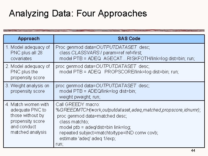
Analyzing Data: Four Approaches Approach SAS Code 1. Model adequacy of Proc genmod data=OUTPUTDATASET desc; PNC plus all 28 class CLASSVARS / param=ref ref=first; covariates model PTB = ADEQ AGECAT…RISKFOTH/link=log dist=bin; run; 2. Model adequacy of proc genmod data=OUTPUTDATASET desc; PNC plus the model PTB = ADEQ PROPSCORE/link=log dist=bin; run; propensity score 3. Weight analysis on propensity score proc genmod data=OUTPUTDATASET desc; model PTB = ADEQ/link=log dist=bin; weight pweight; run; 4. Match women with adequate PNC to those without by propensity score and conduct matched analysis Call GREEDY macro: %GREEDMTCH(work, outputdataset, adeq, matched, propscore, idnumr); proc genmod data=matched desc; class matchto; model ptb = adeq/dist=bin link=log; repeated subject=matchto/type=IND corrw covb; estimate 'adeq' adeq 1/exp; run; 44

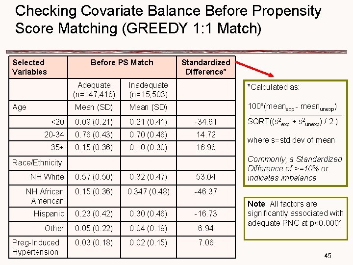
Checking Covariate Balance Before Propensity Score Matching (GREEDY 1: 1 Match) Selected Variables Before PS Match Standardized Difference* Adequate (n=147, 416) Inadequate (n=15, 503) *Calculated as: Mean (SD) 100*(meanexp - meanunexp) <20 0. 09 (0. 21) 0. 21 (0. 41) -34. 61 20 -34 0. 76 (0. 43) 0. 70 (0. 46) 14. 72 35+ 0. 15 (0. 36) 0. 10 (0. 30) 16. 96 Age Race/Ethnicity NH White 0. 57 (0. 50) 0. 32 (0. 47) 53. 04 NH African American 0. 15 (0. 36) 0. 347 (0. 48) -46. 37 Hispanic 0. 23 (0. 42) 0. 30 (0. 46) -16. 73 Other 0. 05 (0. 22) 0. 04 (0. 19) 6. 94 0. 03 (0. 18) 0. 02 (0. 15) 7. 06 Preg-Induced Hypertension SQRT((s 2 exp + s 2 unexp) / 2 ) where s=std dev of mean Commonly, a Standardized Difference of >=10% or indicates imbalance Note: All factors are significantly associated with adequate PNC at p<0. 0001 45

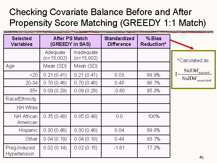
Checking Covariate Balance Before and After Propensity Score Matching (GREEDY 1: 1 Match) Selected Variables After PS Match (GREEDY in SAS) Standardized Difference % Bias Reduction^ Adequate (n=15, 002) Inadequate (n=15, 002) Mean (SD) <20 0. 21 (0. 41) 0. 03 99. 9% 20 -34 0. 70 (0. 46) 0. 48 96. 7% 35+ 0. 09 (0. 29) -0. 80 95. 3% NH African 0. 35 (0. 48) American 0. 35 (0. 48) 0. 0 100% Age ^Calculated as: Race/Ethnicity NH White Hispanic 0. 30 (0. 46) 0. 04 99. 8% Other 0. 04 (0. 19) 0. 04 (0. 18) 0. 44 93. 7% 0. 02 (0. 14) 0. 02 (0. 15) -1. 61 77. 2% Preg-Induced Hypertension 46

Distribution of Propensity Score by PNC Adequacy, after Matching (GREEDY) 47

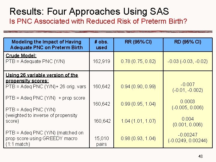
Results: Four Approaches Using SAS Is PNC Associated with Reduced Risk of Preterm Birth? Modeling the Impact of Having Adequate PNC on Preterm Birth # obs. used RR (95% CI) RD (95% CI) Crude Model: PTB = Adequate PNC (Y/N) 162, 919 0. 78 (0. 75, 0. 82) -0. 03 (-0. 03, -0. 02) Using 26 variable version of the propensity scores: PTB = Adeq PNC (Y/N)+ 26 orig. vars 160, 642 0. 94 (0. 90, 0. 99) -0. 007 (-0. 01, -0. 002) 160, 642 0. 99 (0. 95, 1. 04) 0. 0003 (-0. 005, 0. 006) 160, 642 1. 04 (1. 01, 1. 07) 0. 004 (0. 001, 0. 006) 15, 010 pairs 0. 98 (0. 93, 1. 04) -0. 00247 (-0. 0249, 0. 00244) PTB = Adeq PNC (Y/N) + prop score PTB = Adeq PNC (Y/N) (weighted to inverse of propensity score) PTB = Adeq PNC (Y/N) (matched on prop score using GREEDY macro (1: 1 match) 48

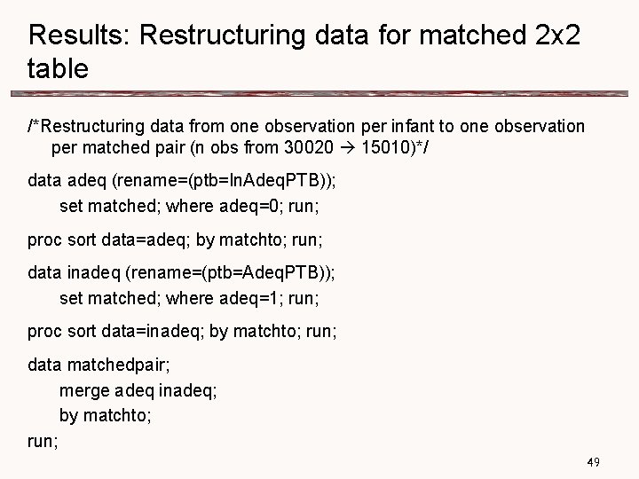
Results: Restructuring data for matched 2 x 2 table /*Restructuring data from one observation per infant to one observation per matched pair (n obs from 30020 15010)*/ data adeq (rename=(ptb=In. Adeq. PTB)); set matched; where adeq=0; run; proc sort data=adeq; by matchto; run; data inadeq (rename=(ptb=Adeq. PTB)); set matched; where adeq=1; run; proc sort data=inadeq; by matchto; run; data matchedpair; merge adeq inadeq; by matchto; run; 49

Results: Matched Analysis from 2 x 2 Table /*Producing 2 x 2 table for matched pairs, with Mc. Nemar test*/ proc freq data=matchedpair order=formatted; table Inadeq. PTB*Adeq. PTB/norow nocol; exact mcnem; format Adeq. PTB Inadeq. PTB yn. ; run; RR = (a+c) / (a+b) SE (ln. RR) = sqrt [(b+c) / {(a+b)(a+c)}] 95% CI = exp[ln. RR ± (1. 96*SE)] RR = (288+1623) / (288+1660) = 0. 981 SE = sqrt [(1660+1623) / {(288+1660)(288+1623)}] = 0. 0297 95% CI = 0. 926, 1. 040

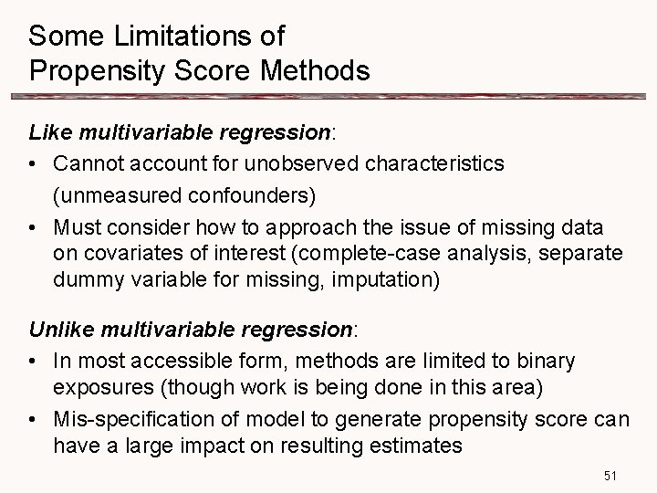
Some Limitations of Propensity Score Methods Like multivariable regression: • Cannot account for unobserved characteristics (unmeasured confounders) • Must consider how to approach the issue of missing data on covariates of interest (complete-case analysis, separate dummy variable for missing, imputation) Unlike multivariable regression: • In most accessible form, methods are limited to binary exposures (though work is being done in this area) • Mis-specification of model to generate propensity score can have a large impact on resulting estimates 51

Some Limitations of Propensity Score Methods Propensity score techniques may not result in different findings than multivariable regression; it’s not always clear that there is a benefit to performing the analysis in this way Some exceptions include: • Datasets in which sample size is limited or the outcome is rare, and multiple covariates need to be controlled; propensity scores provide a way to adjust for all covariates with fewer degrees of freedom • Datasets in which some of the data is off-support; though care must be taken in interpretation as generalizability is affected and, in some cases, bias can be introduced when sample is restricted Sturmer, et al 2006, J Clin Epidemiol. 52

Questions and Challenges 1. What if there is interest in the independent effects of a few other variables besides the 'exposure' – as in any matched design, should these variables not be included in the pool used to create the propensity scores so that they can then be included as covariates in a final model? 53

Questions and Challenges 2. While the model to create the propensity scores can include many variables regardless of their statistical significance, the number of observations lost due to missing values likely increases as the number of variables used increases. What is the balance here? Does this call for imputation? 54

Questions and Challenges 3. For a given sample size, at some point the model to produce the propensity scores will get too big, so although theoretically many variables can be included, mechanically there may be convergence problems. With very small samples, this may mean that fully controlling for observed confounding may not be possible even with propensity scores. With a small number of variables, is it still worth it to gain the efficiency of matching—creating comparable groups. 55

Questions and Challenges 4. One approach to using propensity scores is to weight the observations. Is this possible with a complex sampling design in which the observations are already weighted? 56

Questions and Challenges 5. Choices about level of measurement might be made differently when modeling to generate propensity scores. For example, variables might be left in continuous form even though they might be categorized when assessing their independent effect on outcome (e. g. child's age). Similarly, for categorical variables, there is no need to collapse categories even when modeling results indicate it would be appropriate since parsimony is not critical (e. g. not combining "multiracial" with "other"). 57

Questions and Challenges 6. For stratified analysis, should propensity scores be created first for all observations in a single model (of course not including the stratification variable), or should stratum-specific models be run to create the propensity scores? And, if the scores are generated within strata, should identical pools of variables be used, or might those pools also be stratum-specific ? 58

Resources Software SAS GREEDY MACRO – code and documentation: http: //www 2. sas. com/proceedings/sugi 26/p 214 -26. pdf STATA PSMATCH 2: http: //ideas. repec. org/c/bocode/s 432001. html Other Matching Programs: http: //www. biostat. jhsph. edu/~estuart/propensityscoresoftware. html Select Methods Articles Austin, Peter. Comparing paired vs non-paired statistical methods of analyses when making inferences about absolute risk reductions in propensity-score matched Samples Statist. Med. 2011, 30 1292— 1301. (Plus any other recent Austin papers). Caliendo and Kopeinig , 2005 “Some Practical Guidance for the Implementation of Propensity Score Matching” Available at: http: //repec. iza. org/dp 1588. pdf Oakes JM and Johnson P. Propensity Score Matching for Social Epidemiology. Oakes JM, Kaufman JS (Eds. ), Methods in Social Epidemiology. San Francisco, CA: Jossey-Bass. Stürmer T, Joshi M, Glynn RJ, Avorn J, Rothman KJ, Schneeweiss S. A Review of Propensity Score Methods Yielded Increasing Use, Advantages in Specific Settings, but not Substantially Different Estimates Compared with Conventional Multivariable Methods. J Clin Epidemiol. 2006 May; 59(5): 437 -447. 59

Resources Some MCH Applications Bird TM, Bronstein JM, Hall RW, Lowery CL, Nugent R, Mays GP. Late preterm infants: birth outcomes and health care utilization in the first year. Pediatrics (2): e 311 -9. Epub 2010 Jul 5. Brandt S, Gale S, Tager IB. Estimation of treatment effect of asthma case management using propsensity score methods. Am J Mang Care, 16(4): 257 -64, 2010. Cheng YW, Hubbard A, Caughey AB, Tager IB. The association between persistent fetal occiput posterior position and perinatal outcomes: An example of proensity score and covariate distance matching. AJE, 171(6): 656 -663, 2010. Johnson P, Oakes JM, Anderton DL. Neighborhood Poverty and American Indian Infant Death: Are the Effects Identifiable? Annals of Epidemiology 18(7), 2008: 552 -559. 60