WHATS NEW IN CAUSAL INFERENCE From Propensity Scores

WHAT'S NEW IN CAUSAL INFERENCE: From Propensity Scores And Mediation To External Validity And Selection Bias Judea Pearl UCLA (www. cs. ucla. edu/~judea/) 1

OUTLINE 1. Unified conceptualization of counterfactuals, structural-equations, and graphs 2. Propensity scores demystified 3. Direct and indirect effects (Mediation) 4. External validity mathematized 2

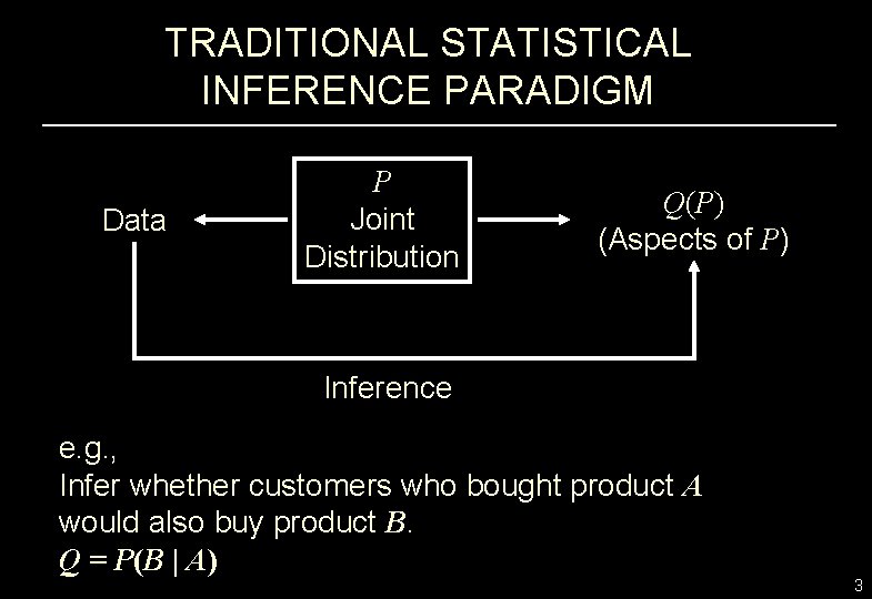
TRADITIONAL STATISTICAL INFERENCE PARADIGM Data P Joint Distribution Q(P) (Aspects of P) Inference e. g. , Infer whether customers who bought product A would also buy product B. Q = P(B | A) 3

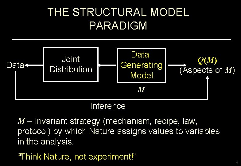
THE STRUCTURAL MODEL PARADIGM Data Joint Distribution Data Generating Model Q(M) (Aspects of M) M Inference M – Invariant strategy (mechanism, recipe, law, protocol) by which Nature assigns values to variables in the analysis. • “Think Nature, not experiment!” 4

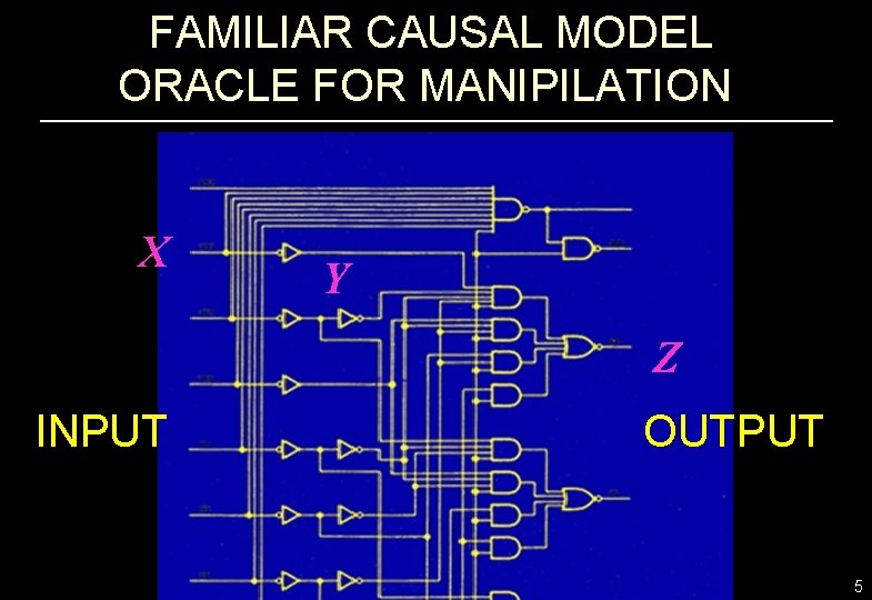
FAMILIAR CAUSAL MODEL ORACLE FOR MANIPILATION X Y Z INPUT OUTPUT 5

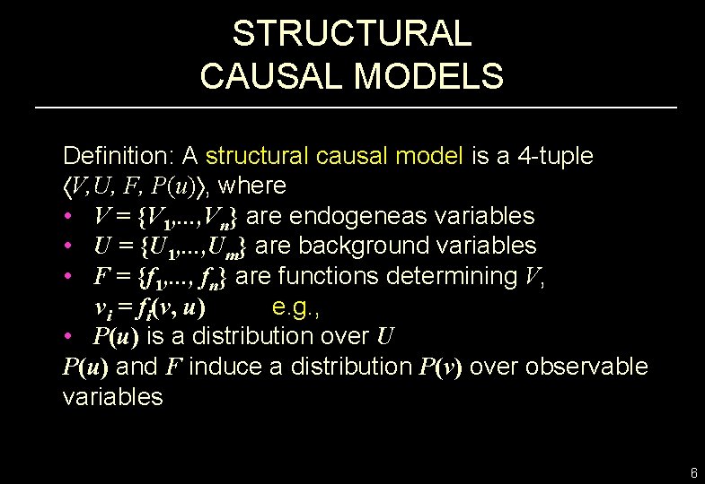
STRUCTURAL CAUSAL MODELS Definition: A structural causal model is a 4 -tuple V, U, F, P(u) , where • V = {V 1, . . . , Vn} are endogeneas variables • U = {U 1, . . . , Um} are background variables • F = {f 1, . . . , fn} are functions determining V, vi = fi(v, u) e. g. , • P(u) is a distribution over U P(u) and F induce a distribution P(v) over observable variables 6

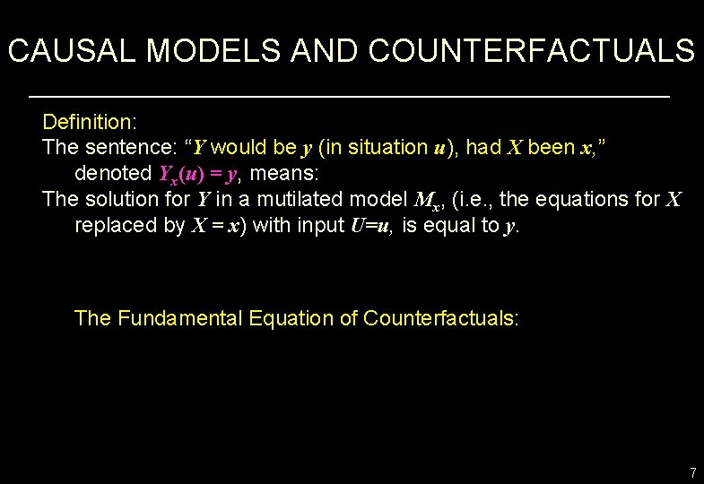
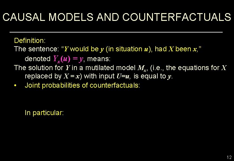
CAUSAL MODELS AND COUNTERFACTUALS Definition: The sentence: “Y would be y (in situation u), had X been x, ” denoted Yx(u) = y, means: The solution for Y in a mutilated model Mx, (i. e. , the equations for X replaced by X = x) with input U=u, is equal to y. The Fundamental Equation of Counterfactuals: 7

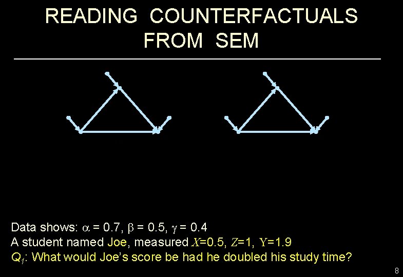
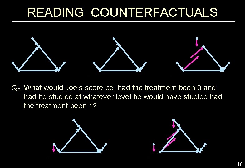
READING COUNTERFACTUALS FROM SEM Data shows: a = 0. 7, b = 0. 5, g = 0. 4 A student named Joe, measured X=0. 5, Z=1, Y=1. 9 Q 1: What would Joe’s score be had he doubled his study time? 8

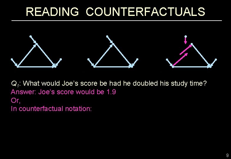
READING COUNTERFACTUALS Q 1: What would Joe’s score be had he doubled his study time? Answer: Joe’s score would be 1. 9 Or, In counterfactual notation: 9

READING COUNTERFACTUALS Q 2: What would Joe’s score be, had the treatment been 0 and had he studied at whatever level he would have studied had the treatment been 1? 10

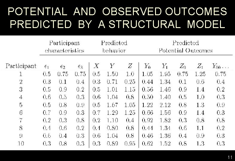
POTENTIAL AND OBSERVED OUTCOMES PREDICTED BY A STRUCTURAL MODEL 11

CAUSAL MODELS AND COUNTERFACTUALS Definition: The sentence: “Y would be y (in situation u), had X been x, ” denoted Yx(u) = y, means: The solution for Y in a mutilated model Mx, (i. e. , the equations for X replaced by X = x) with input U=u, is equal to y. • Joint probabilities of counterfactuals: In particular: 12

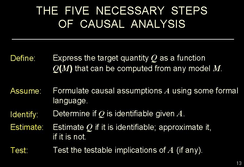
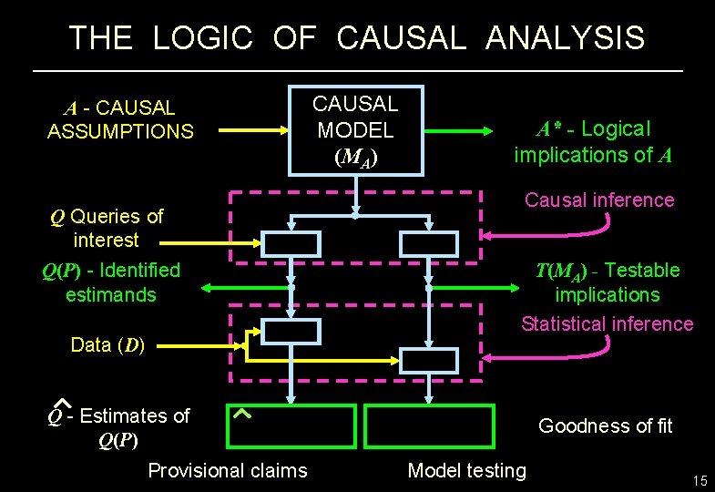
THE FIVE NECESSARY STEPS OF CAUSAL ANALYSIS Define: Express the target quantity Q as a function Q(M) that can be computed from any model M. Assume: Formulate causal assumptions A using some formal language. Identify: Determine if Q is identifiable given A. Estimate: Estimate Q if it is identifiable; approximate it, if it is not. Test: Test the testable implications of A (if any). 13

THE FIVE NECESSARY STEPS OF CAUSAL ANALYSIS Define: Express the target quantity Q as a function Q(M) that can be computed from any model M. Assume: Formulate causal assumptions A using some formal language. Identify: Determine if Q is identifiable given A. Estimate: Estimate Q if it is identifiable; approximate it, if it is not. Test: Test the testable implications of A (if any). 14

THE LOGIC OF CAUSAL ANALYSIS A - CAUSAL ASSUMPTIONS Q Queries of interest Q(P) - Identified estimands Data (D) CAUSAL MODEL (MA) A* - Logical implications of A Causal inference T(MA) - Testable implications Statistical inference Q - Estimates of Q(P) Provisional claims Goodness of fit Model testing 15

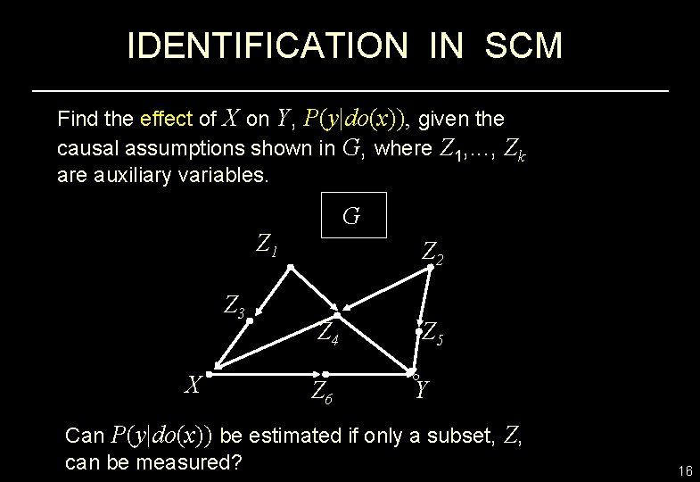
IDENTIFICATION IN SCM Find the effect of X on Y, P(y|do(x)), given the causal assumptions shown in G, where Z 1, . . . , Zk are auxiliary variables. G Z 1 Z 3 X Z 2 Z 4 Z 5 Z 6 Y Can P(y|do(x)) be estimated if only a subset, Z, can be measured? 16

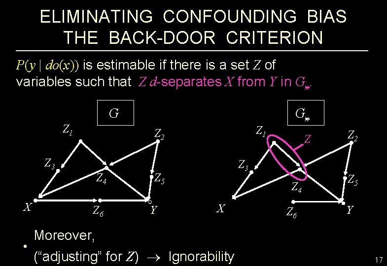
ELIMINATING CONFOUNDING BIAS THE BACK-DOOR CRITERION P(y | do(x)) is estimable if there is a set Z of variables such that Z d-separates X from Y in Gx. G Z 1 • Z 1 Z 2 Z 3 X Gx Z 4 Z 6 Z 3 Z 5 Y Z Z 4 X Z 6 Z 2 Z 5 Y Moreover, (“adjusting” for Z) Ignorability 17

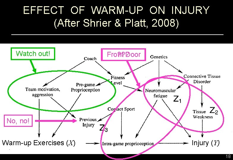
EFFECT OF WARM-UP ON INJURY (After Shrier & Platt, 2008) Watch out! ? ? ? Front Door No, no! Warm-up Exercises (X) Injury (Y) 18

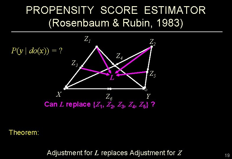
PROPENSITY SCORE ESTIMATOR (Rosenbaum & Rubin, 1983) Z 1 Z 2 P(y | do(x)) = ? Z 4 Z 3 L Z 5 X Z 6 Y Can L replace {Z 1, Z 2, Z 3, Z 4, Z 5} ? Theorem: Adjustment for L replaces Adjustment for Z 19

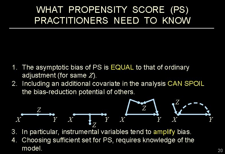
WHAT PROPENSITY SCORE (PS) PRACTITIONERS NEED TO KNOW 1. The asymptotic bias of PS is EQUAL to that of ordinary adjustment (for same Z). 2. Including an additional covariate in the analysis CAN SPOIL the bias-reduction potential of others. Z Z Z X Y X Y Z 3. In particular, instrumental variables tend to amplify bias. 4. Choosing sufficient set for PS, requires knowledge of the model. 20

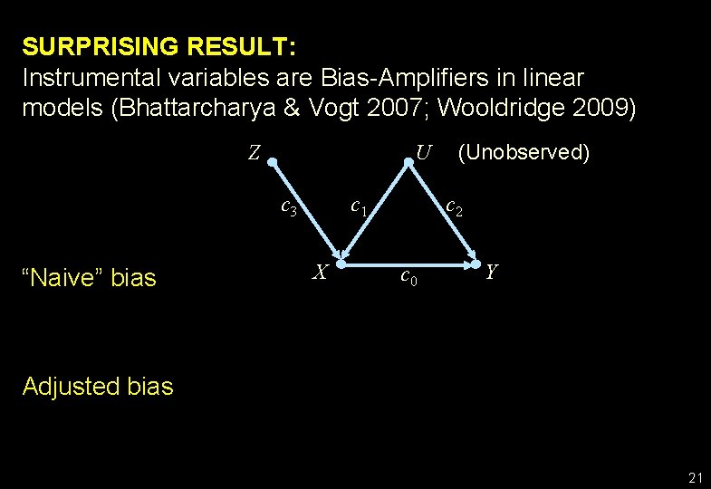
SURPRISING RESULT: Instrumental variables are Bias-Amplifiers in linear models (Bhattarcharya & Vogt 2007; Wooldridge 2009) Z U c 3 “Naive” bias c 1 X (Unobserved) c 2 c 0 Y Adjusted bias 21

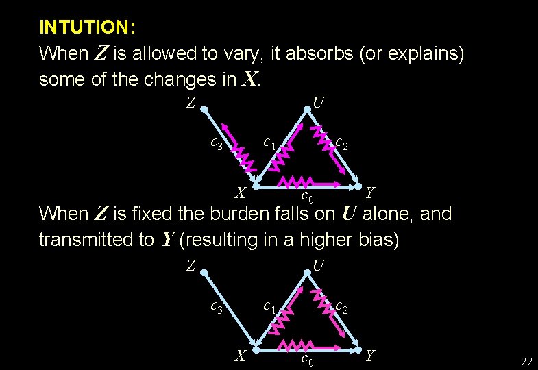
INTUTION: When Z is allowed to vary, it absorbs (or explains) some of the changes in X. Z U c 3 c 1 X c 2 Y c 0 When Z is fixed the burden falls on U alone, and transmitted to Y (resulting in a higher bias) Z U c 3 c 1 X c 2 c 0 Y 22

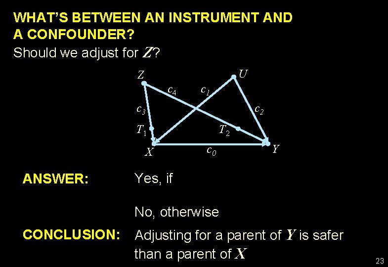
WHAT’S BETWEEN AN INSTRUMENT AND A CONFOUNDER? Should we adjust for Z? U Z c 4 c 1 c 3 c 2 T 1 X T 2 c 0 ANSWER: Yes, if No, otherwise Y CONCLUSION: Adjusting for a parent of Y is safer than a parent of X 23

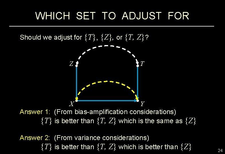
WHICH SET TO ADJUST FOR Should we adjust for {T}, {Z}, or {T, Z}? Z T X Y Answer 1: (From bias-amplification considerations) {T} is better than {T, Z} which is the same as {Z} Answer 2: (From variance considerations) {T} is better than {T, Z} which is better than {Z} 24

CONCLUSIONS • The prevailing practice of adjusting for all covariates, especially those that are good predictors of X (the “treatment assignment, ” Rubin, 2009) is totally misguided. • The “outcome mechanism” is as important, and much safer, from both bias and variance viewpoints • As X-rays are to the surgeon, graphs are for causation 25

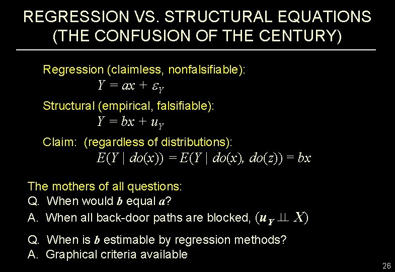
REGRESSION VS. STRUCTURAL EQUATIONS (THE CONFUSION OF THE CENTURY) Regression (claimless, nonfalsifiable): Y = ax + Y Structural (empirical, falsifiable): Y = bx + u. Y Claim: (regardless of distributions): E(Y | do(x)) = E(Y | do(x), do(z)) = bx The mothers of all questions: Q. When would b equal a? A. When all back-door paths are blocked, (u. Y X) Q. When is b estimable by regression methods? A. Graphical criteria available 26

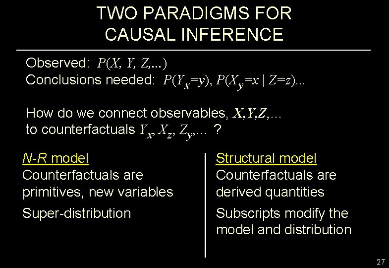
TWO PARADIGMS FOR CAUSAL INFERENCE Observed: P(X, Y, Z, . . . ) Conclusions needed: P(Yx=y), P(Xy=x | Z=z). . . How do we connect observables, X, Y, Z, … to counterfactuals Yx, Xz, Zy, … ? N-R model Counterfactuals are primitives, new variables Structural model Counterfactuals are derived quantities Super-distribution Subscripts modify the model and distribution 27

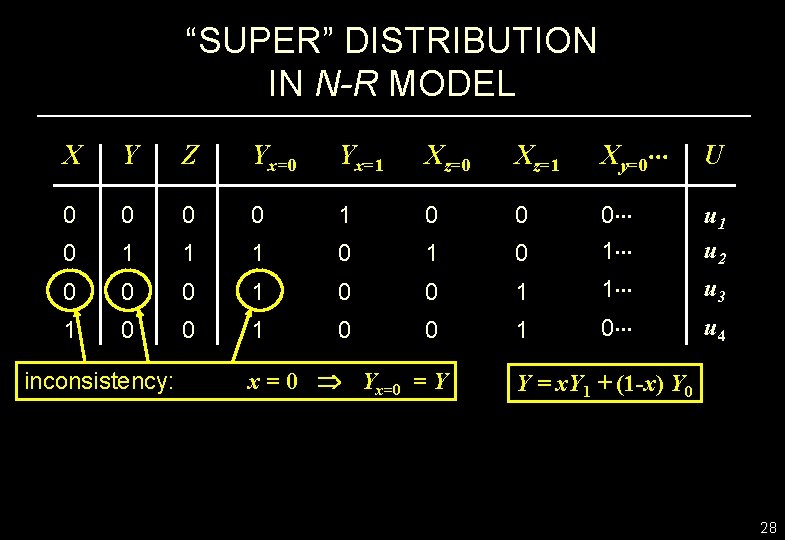
“SUPER” DISTRIBUTION IN N-R MODEL X Y Z Yx=0 Yx=1 Xz=0 Xz=1 Xy=0 U 0 0 1 0 0 0 1 u 2 0 1 1 1 0 0 0 0 1 1 0 0 inconsistency: x = 0 Yx=0 = Y 1 0 u 3 u 4 Y = x. Y 1 + (1 -x) Y 0 28

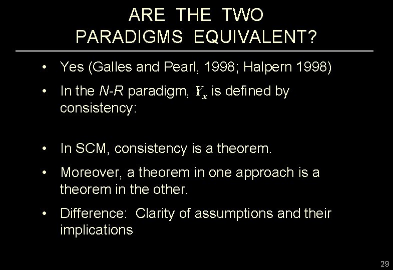
ARE THE TWO PARADIGMS EQUIVALENT? • Yes (Galles and Pearl, 1998; Halpern 1998) • In the N-R paradigm, Yx is defined by consistency: • In SCM, consistency is a theorem. • Moreover, a theorem in one approach is a theorem in the other. • Difference: Clarity of assumptions and their implications 29

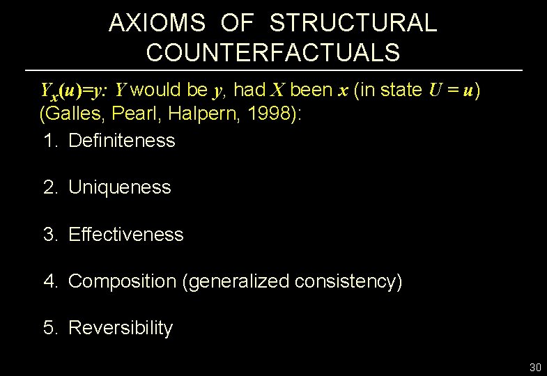
AXIOMS OF STRUCTURAL COUNTERFACTUALS Yx(u)=y: Y would be y, had X been x (in state U = u) (Galles, Pearl, Halpern, 1998): 1. Definiteness 2. Uniqueness 3. Effectiveness 4. Composition (generalized consistency) 5. Reversibility 30

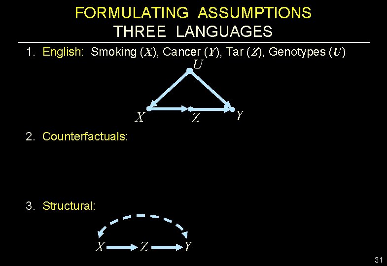
FORMULATING ASSUMPTIONS THREE LANGUAGES 1. English: Smoking (X), Cancer (Y), Tar (Z), Genotypes (U) U X 2. Counterfactuals: Z Y 3. Structural: X Z Y 31

COMPARISON BETWEEN THE N-R AND SCM LANGUAGES 1. Expressing scientific knowledge 2. Recognizing the testable implications of one's assumptions 3. Locating instrumental variables in a system of equations 4. Deciding if two models are equivalent or nested 5. Deciding if two counterfactuals are independent given another 6. Algebraic derivations of identifiable estimands 32

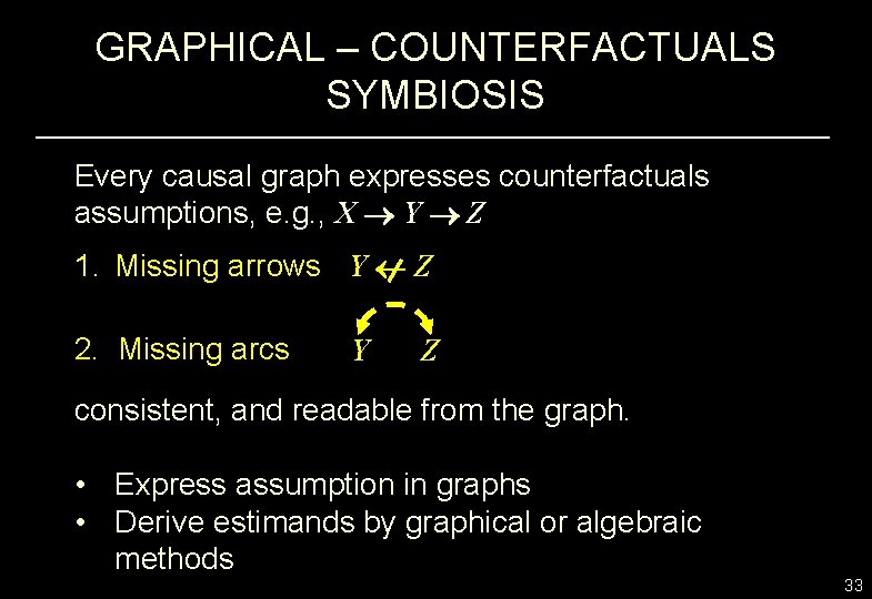
GRAPHICAL – COUNTERFACTUALS SYMBIOSIS Every causal graph expresses counterfactuals assumptions, e. g. , X Y Z 1. Missing arrows Y Z 2. Missing arcs Y Z consistent, and readable from the graph. • Express assumption in graphs • Derive estimands by graphical or algebraic methods 33

EFFECT DECOMPOSITION (direct vs. indirect effects) 1. Why decompose effects? 2. What is the definition of direct and indirect effects? 3. What are the policy implications of direct and indirect effects? 4. When can direct and indirect effect be estimated consistently from experimental and nonexperimental data? 34

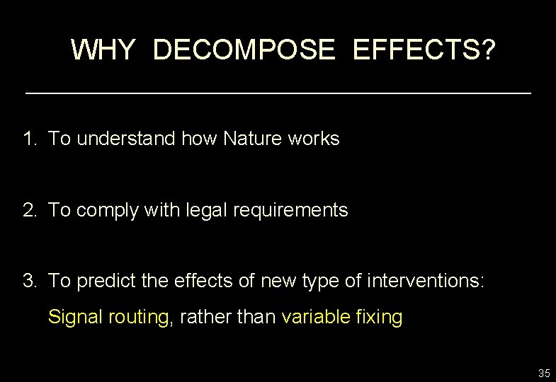
WHY DECOMPOSE EFFECTS? 1. To understand how Nature works 2. To comply with legal requirements 3. To predict the effects of new type of interventions: Signal routing, rather than variable fixing 35

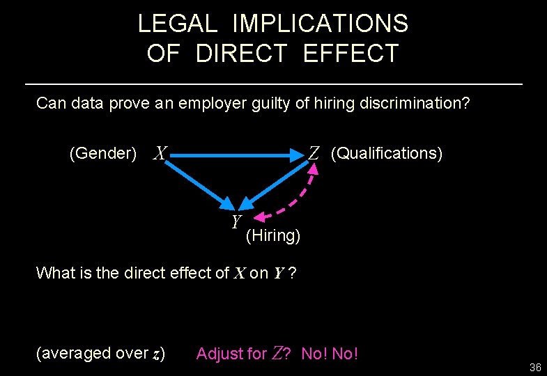
LEGAL IMPLICATIONS OF DIRECT EFFECT Can data prove an employer guilty of hiring discrimination? (Gender) X Z (Qualifications) Y (Hiring) What is the direct effect of X on Y ? (averaged over z) Adjust for Z? No! 36

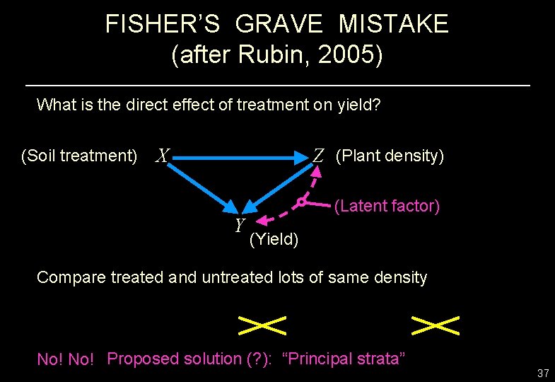
FISHER’S GRAVE MISTAKE (after Rubin, 2005) What is the direct effect of treatment on yield? (Soil treatment) X Z (Plant density) Y (Latent factor) (Yield) Compare treated and untreated lots of same density No! Proposed solution (? ): “Principal strata” 37

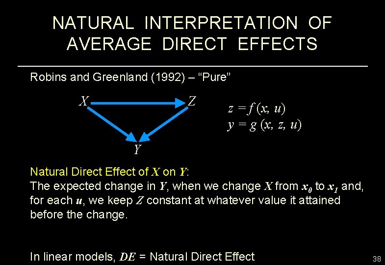
NATURAL INTERPRETATION OF AVERAGE DIRECT EFFECTS Robins and Greenland (1992) – “Pure” X Z z = f (x, u) y = g (x, z, u) Y Natural Direct Effect of X on Y: The expected change in Y, when we change X from x 0 to x 1 and, for each u, we keep Z constant at whatever value it attained before the change. In linear models, DE = Natural Direct Effect 38

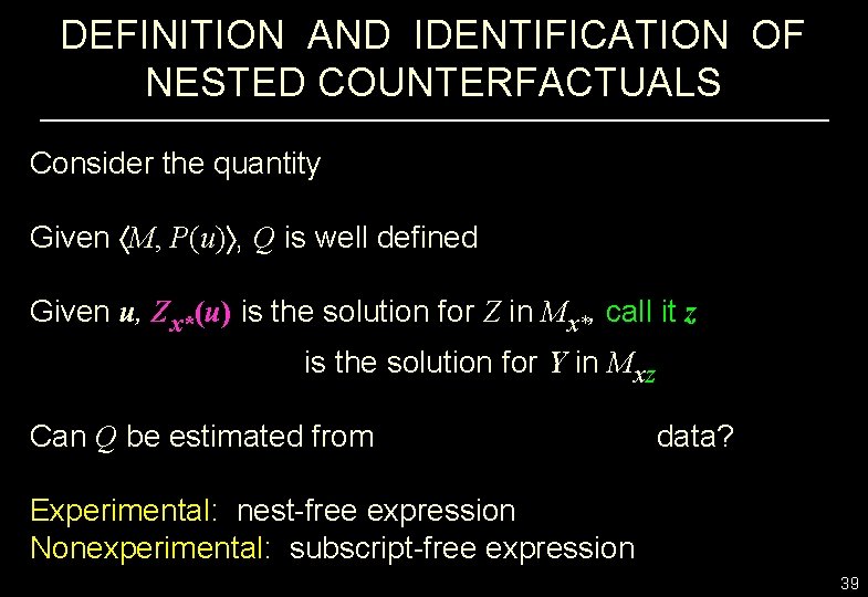
DEFINITION AND IDENTIFICATION OF NESTED COUNTERFACTUALS Consider the quantity Given M, P(u) , Q is well defined Given u, Zx*(u) is the solution for Z in Mx*, call it z is the solution for Y in Mxz Can Q be estimated from data? Experimental: nest-free expression Nonexperimental: subscript-free expression 39

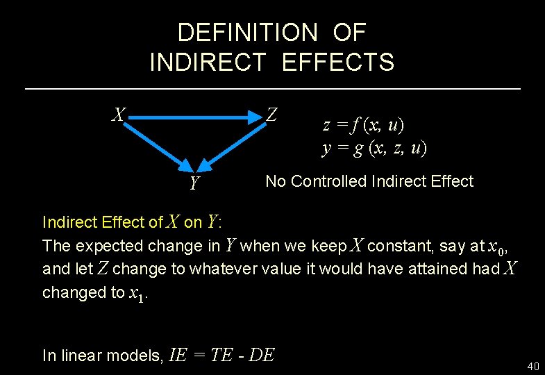
DEFINITION OF INDIRECT EFFECTS X Z Y z = f (x, u) y = g (x, z, u) No Controlled Indirect Effect of X on Y: The expected change in Y when we keep X constant, say at x 0, and let Z change to whatever value it would have attained had X changed to x 1. In linear models, IE = TE - DE 40

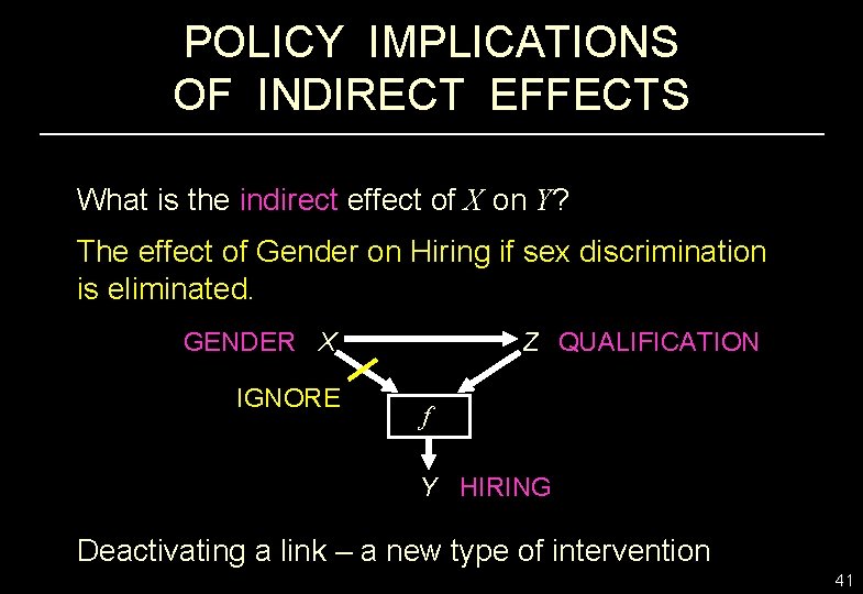
POLICY IMPLICATIONS OF INDIRECT EFFECTS What is the indirect effect of X on Y? The effect of Gender on Hiring if sex discrimination is eliminated. GENDER X IGNORE Z QUALIFICATION f Y HIRING Deactivating a link – a new type of intervention 41

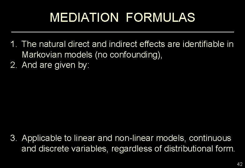
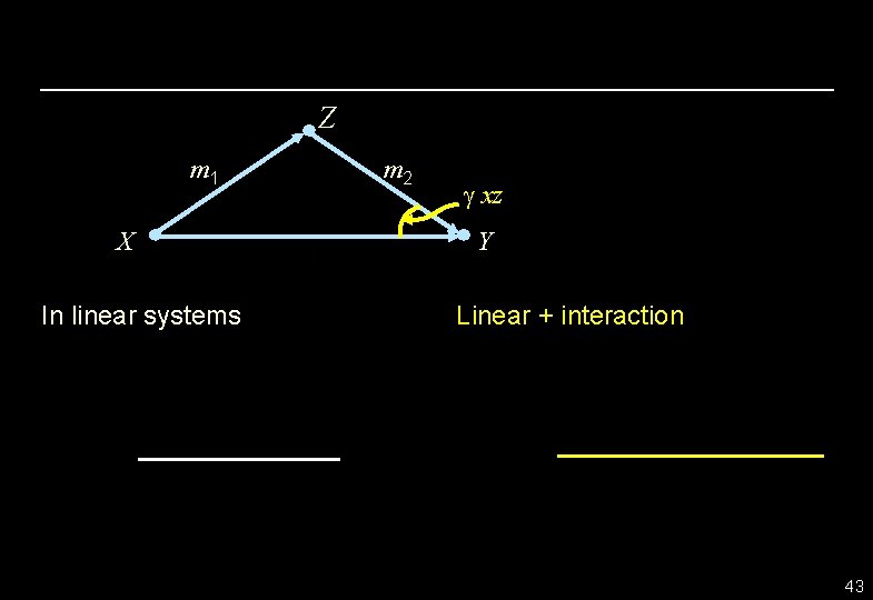
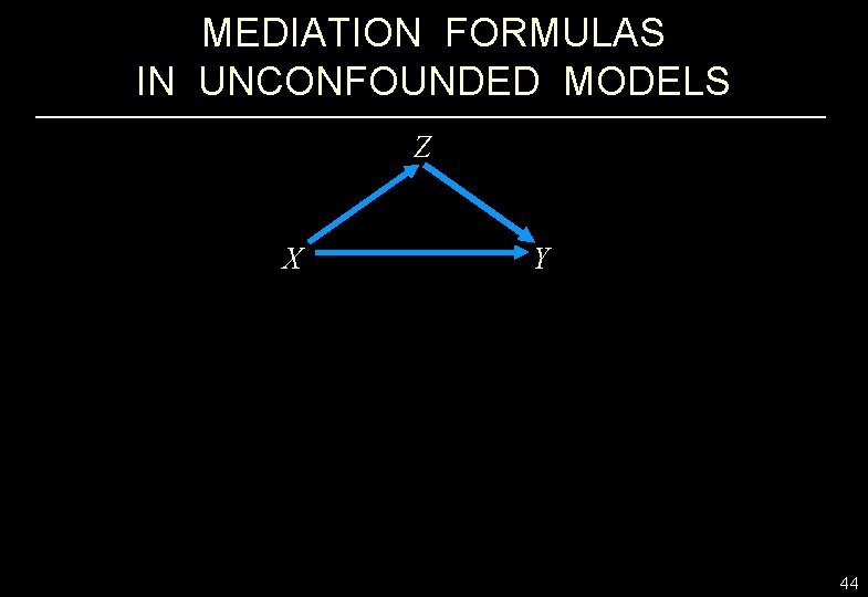
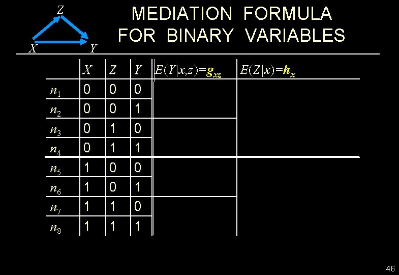
MEDIATION FORMULAS 1. The natural direct and indirect effects are identifiable in Markovian models (no confounding), 2. And are given by: 3. Applicable to linear and non-linear models, continuous and discrete variables, regardless of distributional form. 42

Z m 1 X In linear systems m 2 g xz Y Linear + interaction 43

MEDIATION FORMULAS IN UNCONFOUNDED MODELS Z X Y 44

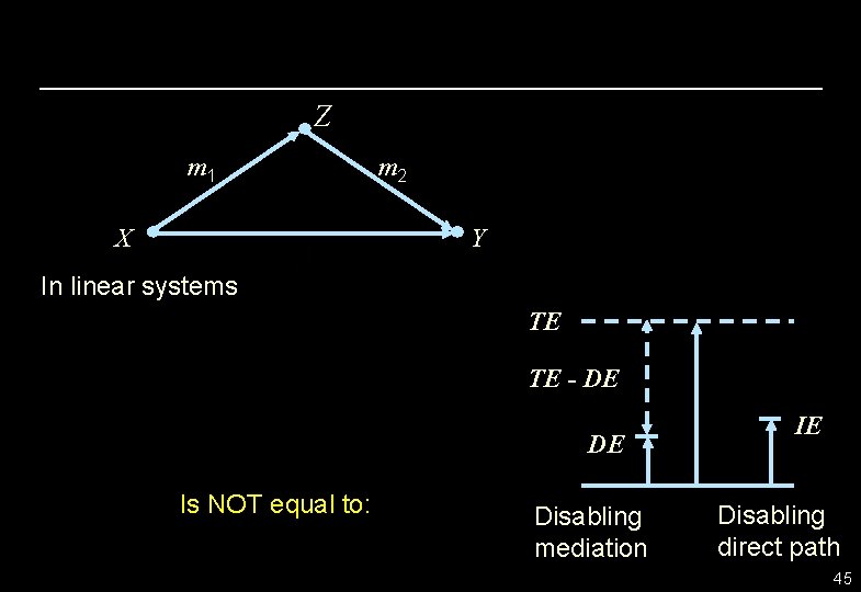
Z m 1 X m 2 Y In linear systems TE TE - DE DE Is NOT equal to: Disabling mediation IE Disabling direct path 45

Z X MEDIATION FORMULA FOR BINARY VARIABLES Y n 1 n 2 n 3 n 4 n 5 n 6 n 7 n 8 X 0 0 1 1 Z 0 0 1 1 Y 0 1 0 1 E(Y|x, z)=gxz E(Z|x)=hx 46

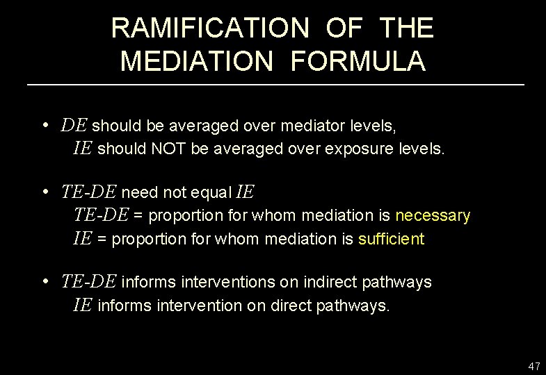
RAMIFICATION OF THE MEDIATION FORMULA • DE should be averaged over mediator levels, IE should NOT be averaged over exposure levels. • TE-DE need not equal IE TE-DE = proportion for whom mediation is necessary IE = proportion for whom mediation is sufficient • TE-DE informs interventions on indirect pathways IE informs intervention on direct pathways. 47

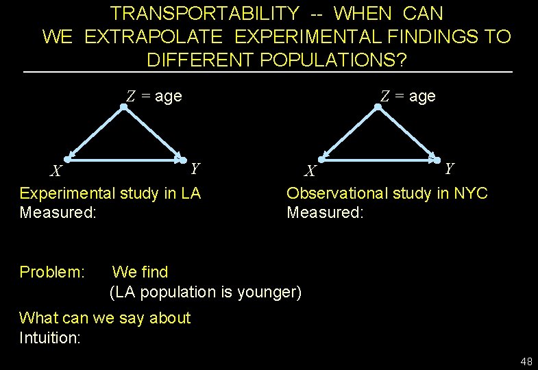
TRANSPORTABILITY -- WHEN CAN WE EXTRAPOLATE EXPERIMENTAL FINDINGS TO DIFFERENT POPULATIONS? Z = age Y X Experimental study in LA Measured: Z = age Y X Observational study in NYC Measured: Problem: We find (LA population is younger) What can we say about Intuition: 48

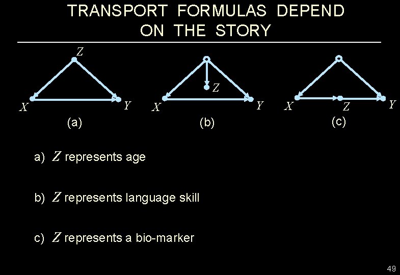
TRANSPORT FORMULAS DEPEND ON THE STORY Z Z Y X (a) (b) X Z (c) Y a) Z represents age b) Z represents language skill c) Z represents a bio-marker 49

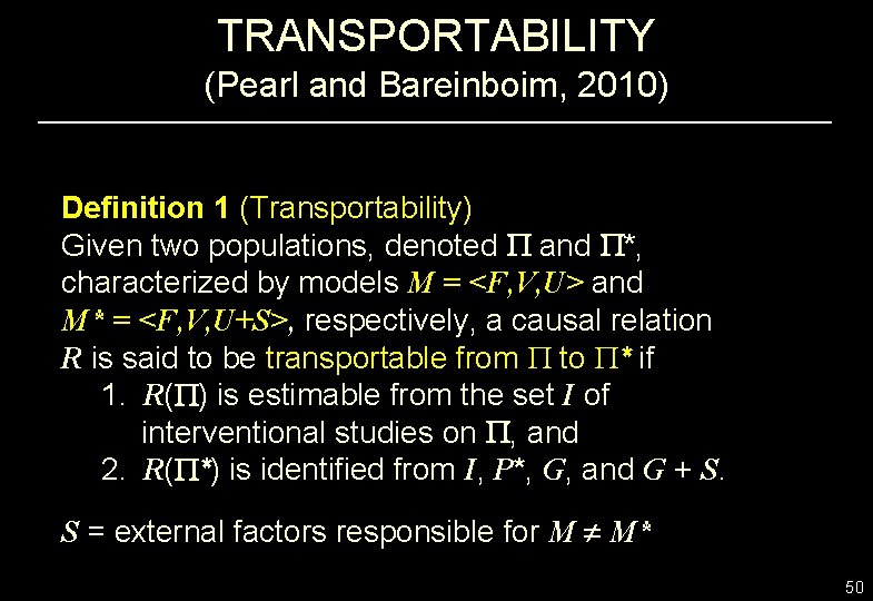
TRANSPORTABILITY (Pearl and Bareinboim, 2010) Definition 1 (Transportability) Given two populations, denoted and *, characterized by models M = <F, V, U> and M* = <F, V, U+S>, respectively, a causal relation R is said to be transportable from to * if 1. R( ) is estimable from the set I of interventional studies on , and 2. R( *) is identified from I, P*, G, and G + S. S = external factors responsible for M M* 50

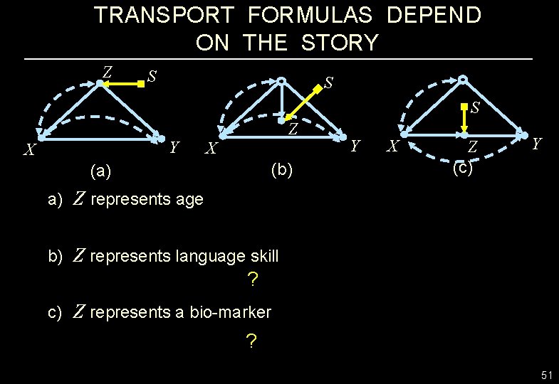
TRANSPORT FORMULAS DEPEND ON THE STORY Z S S S Y X Z X (b) (a) Y X Z (c) Y a) Z represents age b) Z represents language skill ? c) Z represents a bio-marker ? 51

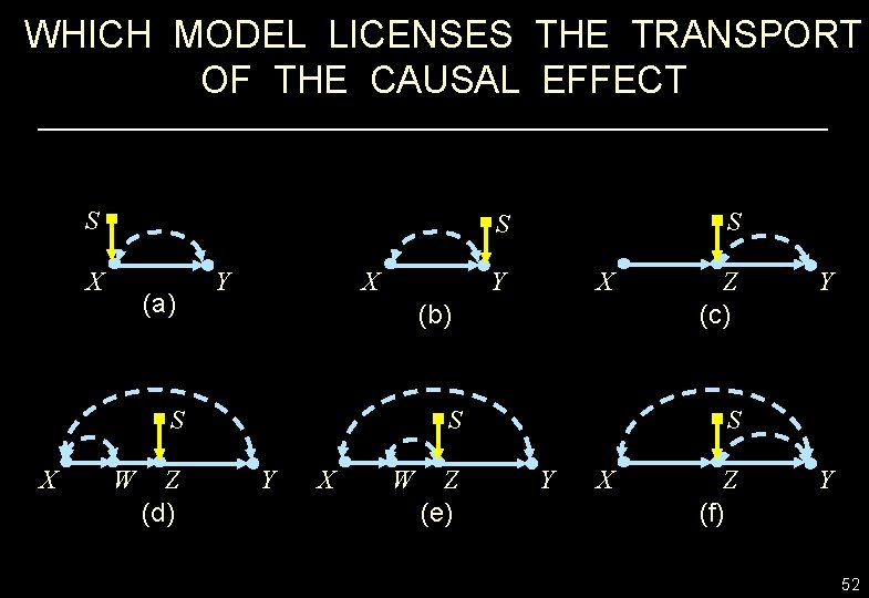
WHICH MODEL LICENSES THE TRANSPORT OF THE CAUSAL EFFECT S X (a) X Y Y W Z (d) X (b) S X S S S Y X W Z (e) Z (c) Y S Y X Z (f) Y 52

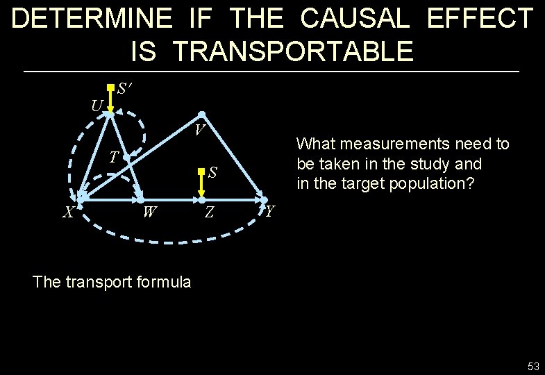
DETERMINE IF THE CAUSAL EFFECT IS TRANSPORTABLE U S V T X What measurements need to be taken in the study and in the target population? S W Z Y The transport formula 53

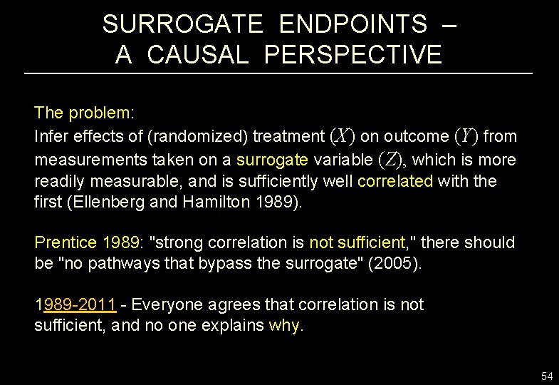
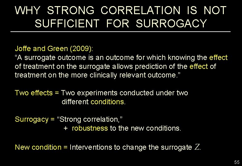
SURROGATE ENDPOINTS – A CAUSAL PERSPECTIVE The problem: Infer effects of (randomized) treatment (X) on outcome (Y) from measurements taken on a surrogate variable (Z), which is more readily measurable, and is sufficiently well correlated with the first (Ellenberg and Hamilton 1989). Prentice 1989: "strong correlation is not sufficient, " there should be "no pathways that bypass the surrogate" (2005). 1989 -2011 - Everyone agrees that correlation is not sufficient, and no one explains why. 54

WHY STRONG CORRELATION IS NOT SUFFICIENT FOR SURROGACY Joffe and Green (2009): “A surrogate outcome is an outcome for which knowing the effect of treatment on the surrogate allows prediction of the effect of treatment on the more clinically relevant outcome. ” Two effects = Two experiments conducted under two different conditions. Surrogacy = “Strong correlation, ” + robustness to the new conditions. New condition = Interventions to change the surrogate Z. 55

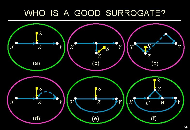
WHO IS A GOOD SURROGATE? S X Z Y X S Z (d) Y X Z (b) (a) X S S Y Z (c) S Z S Y X Z (e) Y X W U Y (f) 56

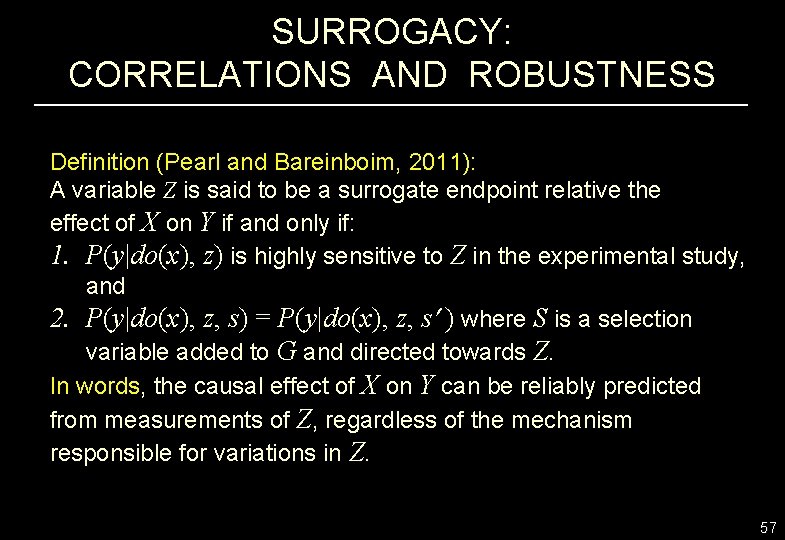
SURROGACY: CORRELATIONS AND ROBUSTNESS Definition (Pearl and Bareinboim, 2011): A variable Z is said to be a surrogate endpoint relative the effect of X on Y if and only if: 1. P(y|do(x), z) is highly sensitive to Z in the experimental study, and 2. P(y|do(x), z, s) = P(y|do(x), z, s ) where S is a selection variable added to G and directed towards Z. In words, the causal effect of X on Y can be reliably predicted from measurements of Z, regardless of the mechanism responsible for variations in Z. 57

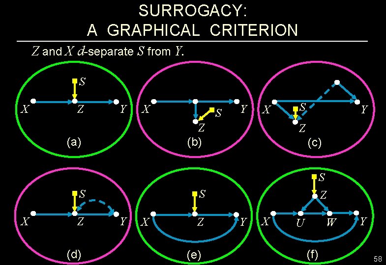
SURROGACY: A GRAPHICAL CRITERION Z and X d-separate S from Y. S X Z Y X S Z (d) Y X Z (b) (a) X S S Y Z (c) S Z S Y X Z (e) Y X W U (f) Y 58

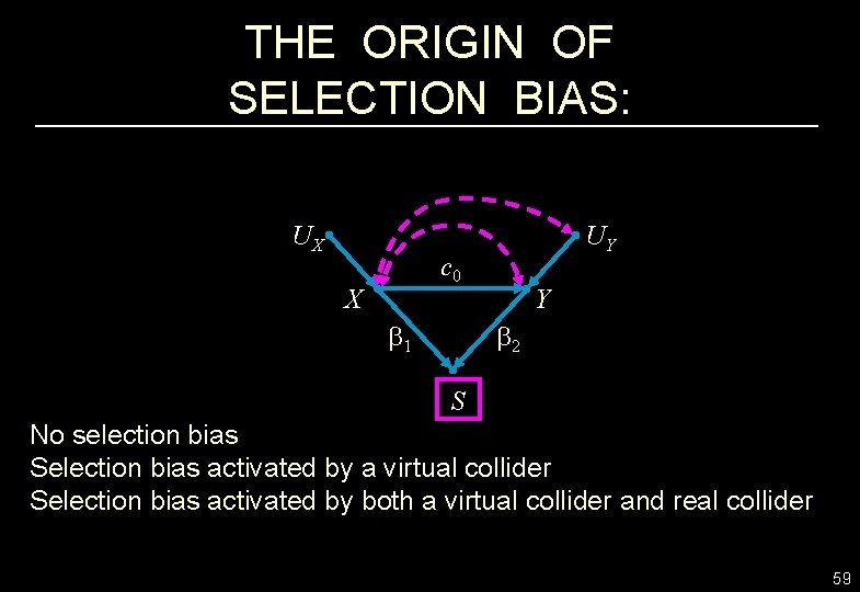
THE ORIGIN OF SELECTION BIAS: UX UY c 0 X b 1 Y b 2 S No selection bias Selection bias activated by a virtual collider Selection bias activated by both a virtual collider and real collider 59

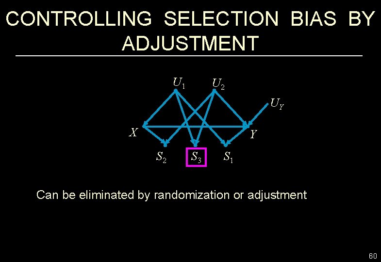
CONTROLLING SELECTION BIAS BY ADJUSTMENT U 1 U 2 UY X Y S 2 S 3 S 1 Can be eliminated by randomization or adjustment 60

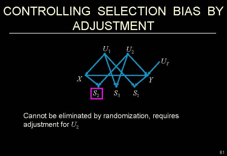
CONTROLLING SELECTION BIAS BY ADJUSTMENT U 1 U 2 UY X Y S 2 S 3 S 1 Cannot be eliminated by randomization, requires adjustment for U 2 61

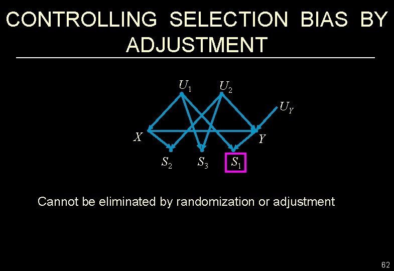
CONTROLLING SELECTION BIAS BY ADJUSTMENT U 1 U 2 UY X Y S 2 S 3 S 1 Cannot be eliminated by randomization or adjustment 62

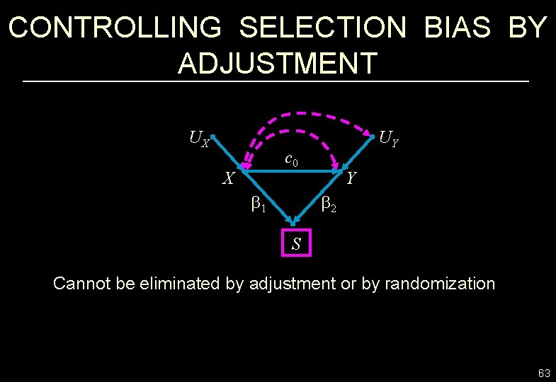
CONTROLLING SELECTION BIAS BY ADJUSTMENT UX UY c 0 X b 1 Y b 2 S Cannot be eliminated by adjustment or by randomization 63

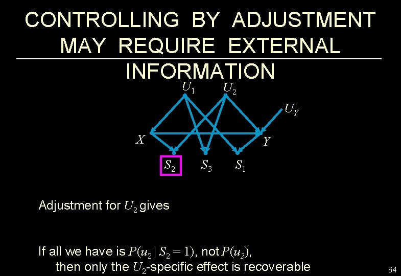
CONTROLLING BY ADJUSTMENT MAY REQUIRE EXTERNAL INFORMATION U 1 U 2 UY X Y S 2 S 3 S 1 Adjustment for U 2 gives If all we have is P(u 2 | S 2 = 1), not P(u 2), then only the U 2 -specific effect is recoverable 64

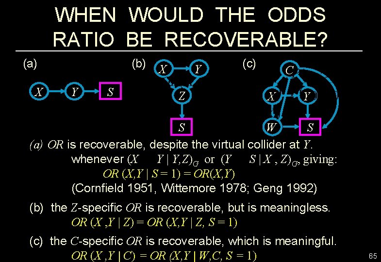
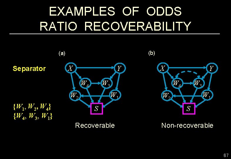
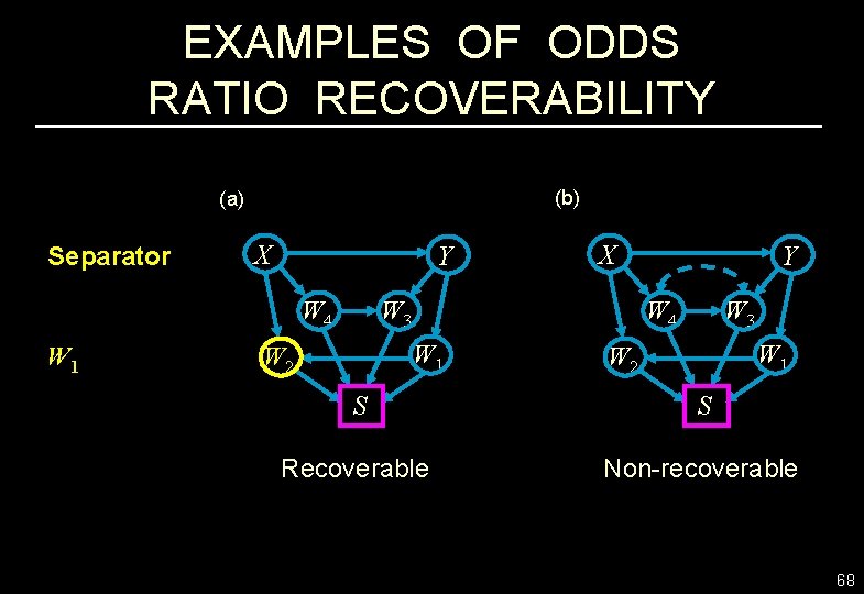
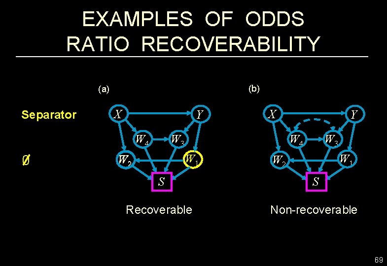
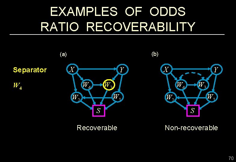
WHEN WOULD THE ODDS RATIO BE RECOVERABLE? (a) (b) X Y S X Y Z (c) C X Y S W S (a) OR is recoverable, despite the virtual collider at Y. whenever (X Y | Y, Z)G or (Y S | X , Z)G, giving: OR (X, Y | S = 1) = OR(X, Y) (Cornfield 1951, Wittemore 1978; Geng 1992) (b) the Z-specific OR is recoverable, but is meaningless. OR (X , Y | Z) = OR (X, Y | Z, S = 1) (c) the C-specific OR is recoverable, which is meaningful. OR (X , Y | C) = OR (X, Y | W, C, S = 1) 65

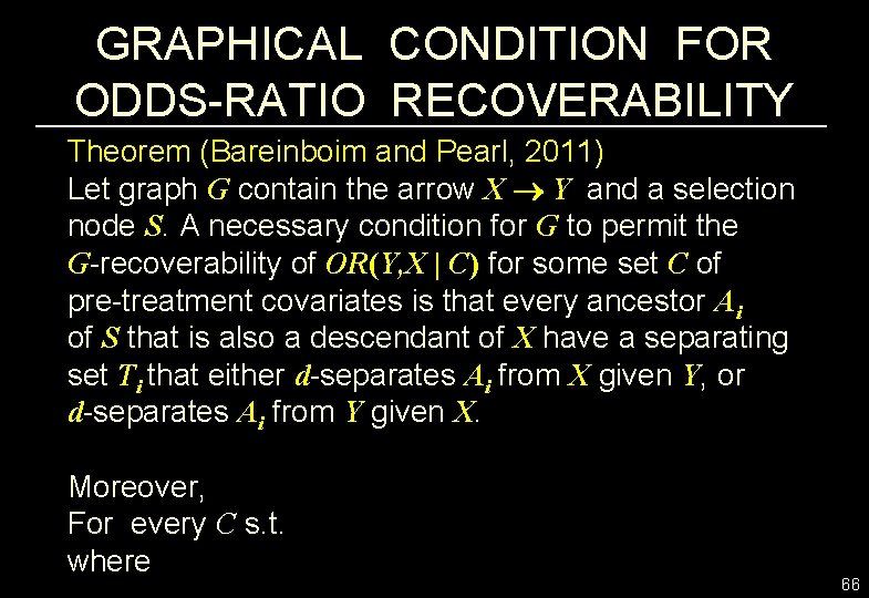
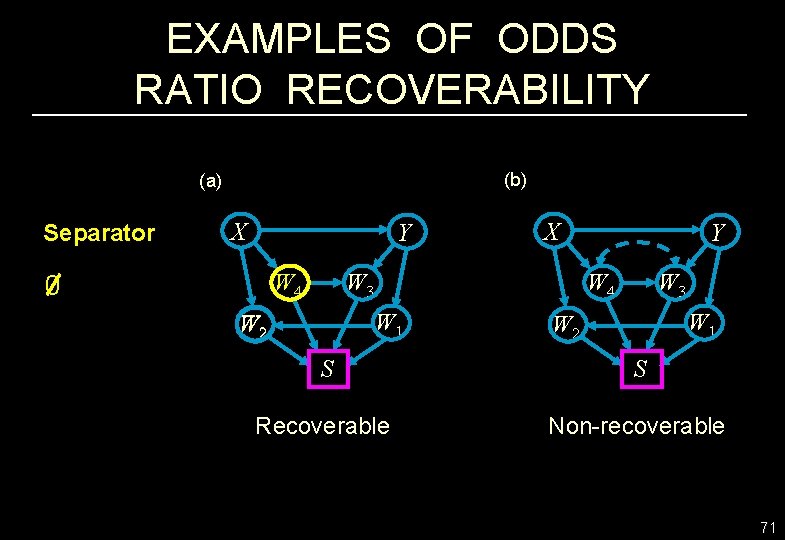
GRAPHICAL CONDITION FOR ODDS-RATIO RECOVERABILITY Theorem (Bareinboim and Pearl, 2011) Let graph G contain the arrow X Y and a selection node S. A necessary condition for G to permit the G-recoverability of OR(Y, X | C) for some set C of pre-treatment covariates is that every ancestor Ai of S that is also a descendant of X have a separating set Ti that either d-separates Ai from X given Y, or d-separates Ai from Y given X. Moreover, For every C s. t. where 66

EXAMPLES OF ODDS RATIO RECOVERABILITY (b) (a) Separator X Y W 4 W 3 Y W 3 W 4 W 1 W 2 {W 1, W 2, W 4} {W 4, W 3, W 1} X W 1 W 2 S S Recoverable Non-recoverable 67

EXAMPLES OF ODDS RATIO RECOVERABILITY (b) (a) Separator X Y W 4 W 1 X W 3 W 4 W 1 W 2 Y W 1 W 2 S S Recoverable Non-recoverable 68

EXAMPLES OF ODDS RATIO RECOVERABILITY (b) (a) Separator X Y W 4 0 X W 3 W 4 W 1 W 2 Y W 1 W 2 S S Recoverable Non-recoverable 69

EXAMPLES OF ODDS RATIO RECOVERABILITY (b) (a) Separator X Y W 4 X W 3 W 4 W 1 W 2 Y W 1 W 2 S S Recoverable Non-recoverable 70

EXAMPLES OF ODDS RATIO RECOVERABILITY (b) (a) Separator X Y W 4 0 X W 3 W 4 W 1 W 2 Y W 1 W 2 S S Recoverable Non-recoverable 71

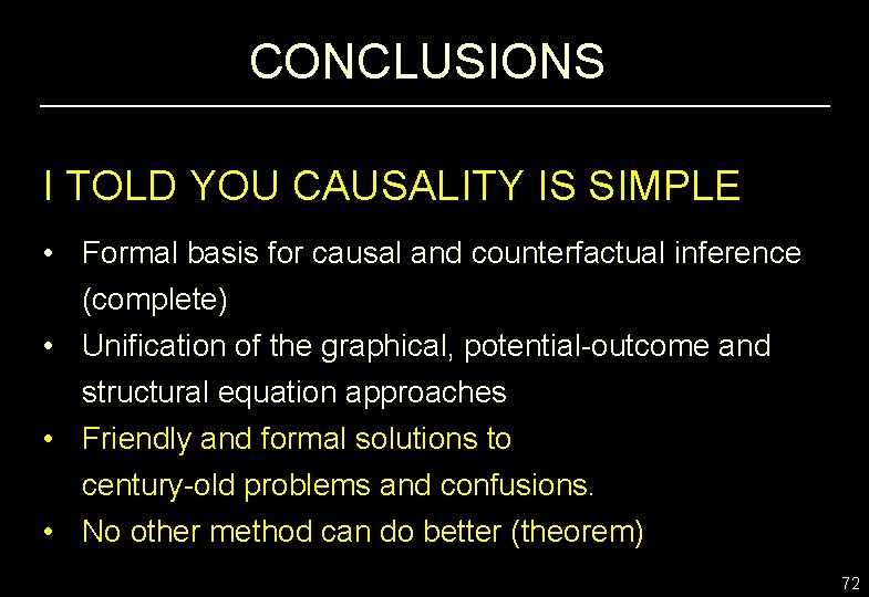
CONCLUSIONS I TOLD YOU CAUSALITY IS SIMPLE • Formal basis for causal and counterfactual inference (complete) • Unification of the graphical, potential-outcome and structural equation approaches • Friendly and formal solutions to century-old problems and confusions. • No other method can do better (theorem) 72

Thank you for agreeing with everything I said. 73