Matching Methods Propensity Scores Garret Christensen Taken from

Matching Methods & Propensity Scores Garret Christensen (Taken from Kenny Ajayi) October 27, 2009 Global Poverty and Impact Evaluation

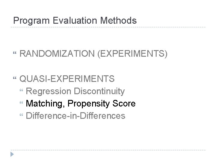
Program Evaluation Methods RANDOMIZATION (EXPERIMENTS) QUASI-EXPERIMENTS Regression Discontinuity Matching, Propensity Score Difference-in-Differences

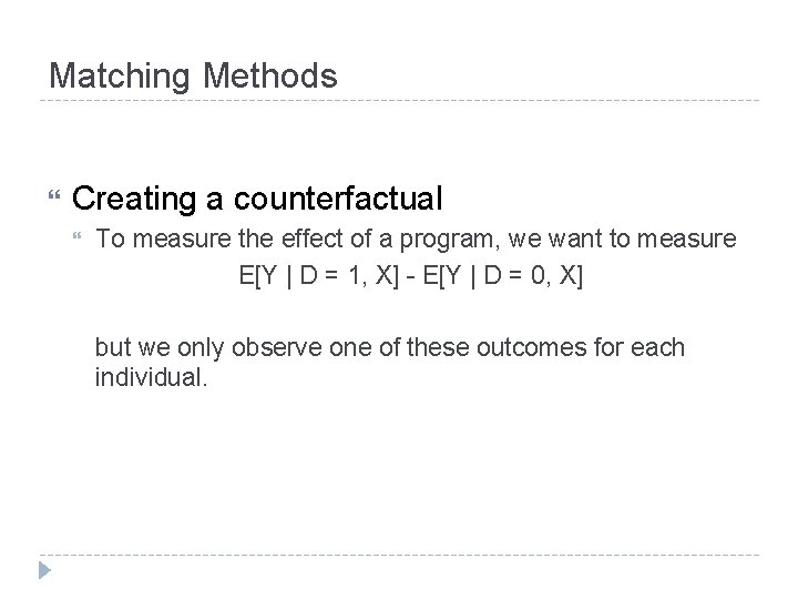
Matching Methods Creating a counterfactual To measure the effect of a program, we want to measure E[Y | D = 1, X] - E[Y | D = 0, X] but we only observe one of these outcomes for each individual.

Evaluation Exercise Argentine Antipoverty Program

Basic Idea Match each participant (treated) with one or more nonparticipants (untreated) with similar observed characteristics Counterfactual = matched comparison group (i. e. nonparticipants with same characteristics as participants) Illustrate Example

Basic Idea This assumes that there is no selection bias based on unobserved characteristics i. e. there is “selection on observables” and participation is independent of outcomes once we control for observable characteristics (X) What might some of these unobserved characteristics be?

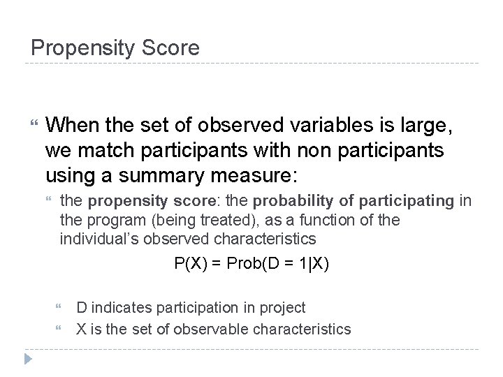
Propensity Score When the set of observed variables is large, we match participants with non participants using a summary measure: the propensity score: the probability of participating in the program (being treated), as a function of the individual’s observed characteristics P(X) = Prob(D = 1|X) D indicates participation in project X is the set of observable characteristics

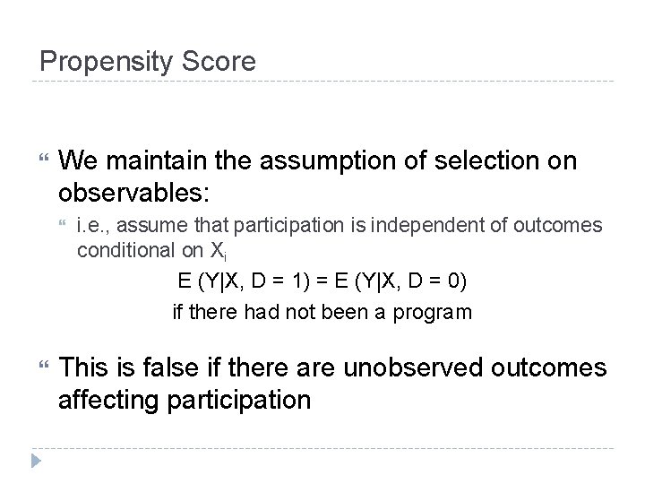
Propensity Score We maintain the assumption of selection on observables: i. e. , assume that participation is independent of outcomes conditional on Xi E (Y|X, D = 1) = E (Y|X, D = 0) if there had not been a program This is false if there are unobserved outcomes affecting participation

Evaluation Exercise Argentine Antipoverty Program

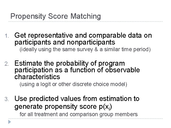
Propensity Score Matching 1. Get representative and comparable data on participants and nonparticipants (ideally using the same survey & a similar time period)

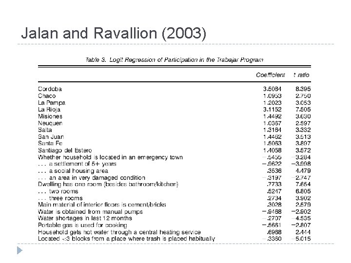
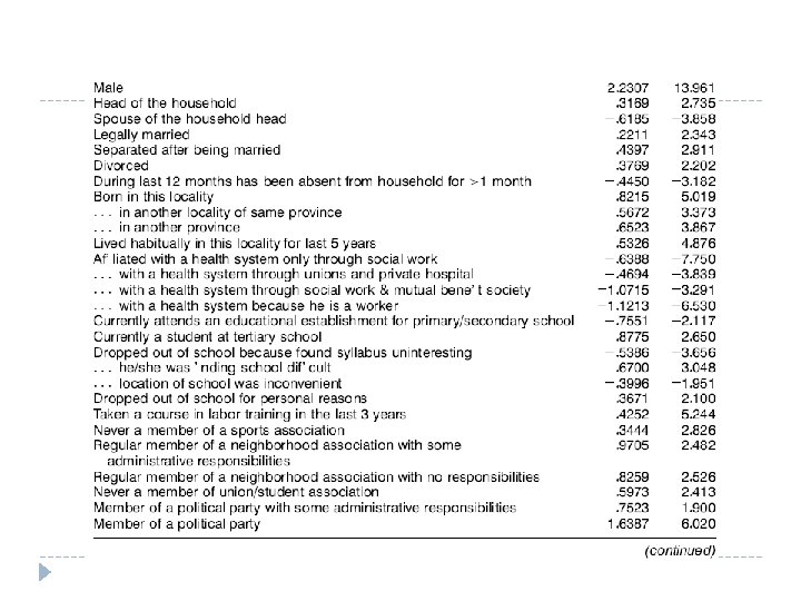
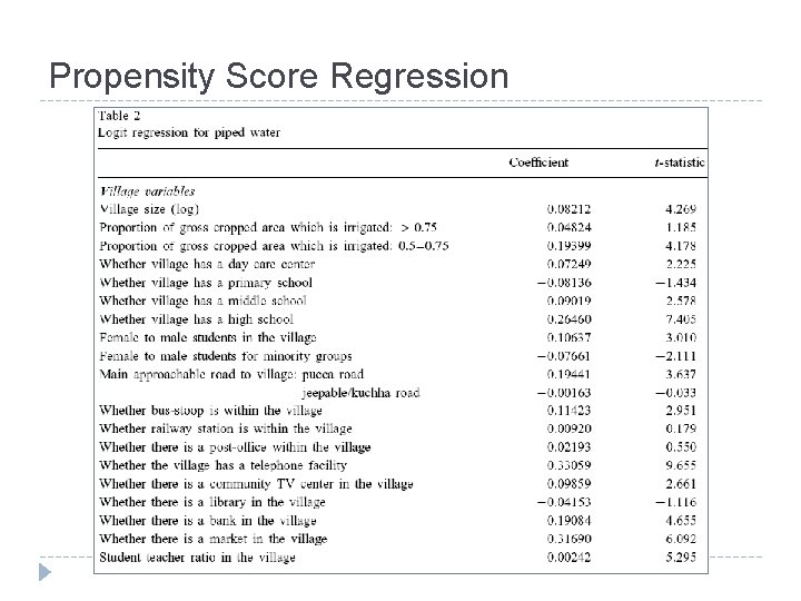
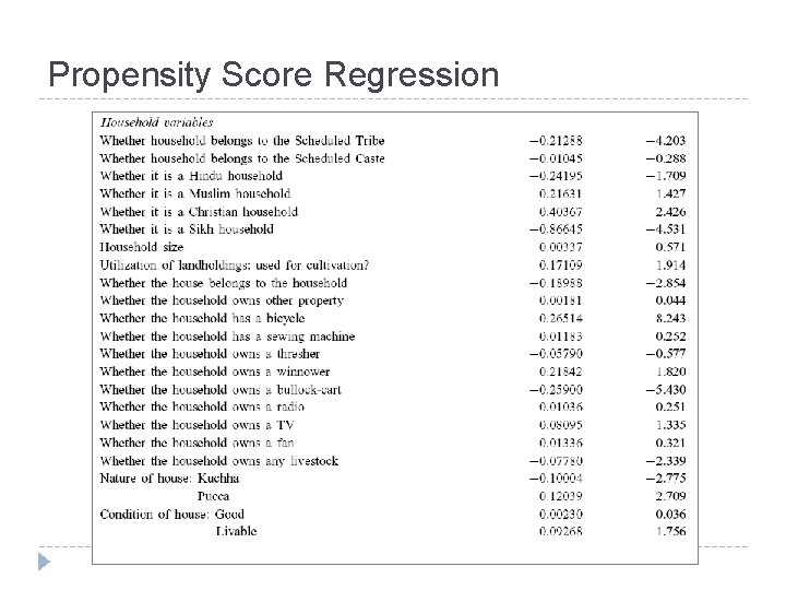
Propensity Score Matching 1. Get representative and comparable data on participants and nonparticipants (ideally using the same survey & a similar time period) 2. Estimate the probability of program participation as a function of observable characteristics (using a logit or other discrete choice model)

Jalan and Ravallion (2003)

Propensity Score Matching 1. Get representative and comparable data on participants and nonparticipants (ideally using the same survey & a similar time period) 2. Estimate the probability of program participation as a function of observable characteristics (using a logit or other discrete choice model) 3. Use predicted values from estimation to generate propensity score p(xi) for all treatment and comparison group members

Propensity Score Matching Match Participants: Find a sample of non- 4. participants with similar p(xi) Restrict samples to ensure common support

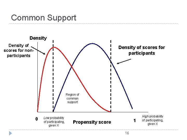
Common Support Density of scores for nonparticipants Density of scores for participants Region of common support 0 Low probability of participating, given X 1 Propensity score 16 High probability of participating, given X

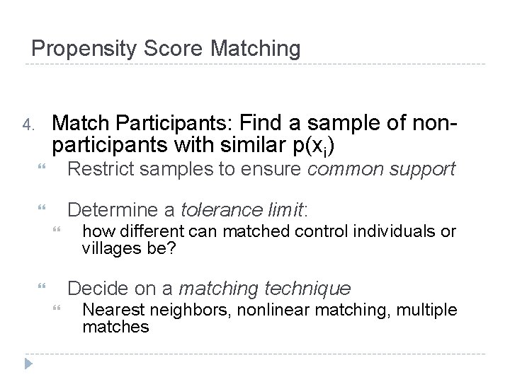
Propensity Score Matching Match Participants: Find a sample of non- 4. participants with similar p(xi) Restrict samples to ensure common support Determine a tolerance limit: how different can matched control individuals or villages be? Decide on a matching technique Nearest neighbors, nonlinear matching, multiple matches

Propensity Score Matching Once matches are made, we can calculate impact by comparing the means of outcomes across participants and their matches 5. The difference in outcomes for each participant and its match is the estimate of the gain due to the program for that observation. Calculate the mean of these individual gains to obtain the average overall gain.

Possible Scenarios Case 1: Baseline Data Exists Arrive at baseline, we can match participants with nonparticipants using baseline characteristics. Case 2: No Baseline Data. Arrive afterwards, we can only match participants with nonparticipants using time-invariant characteristics.

Extensions Be cautious of ex-post matching Matching on variables that change due to program participation (i. e. endogenous variables) What are some invariable characteristics?

Key Factors Identification Assumption Selection on Observables: After controlling for observables, treated and control groups are not systematically different Data Requirements Rich data on as many observable characteristics as possible Large sample size (so that it is possible to find appropriate match)

Additional Considerations Advantages Might be possible to do with existing survey data Doesn’t require randomization/experiment/baseline data Allows estimation of heterogeneous treatment effects because we have individual counterfactuals, instead of just having group averages.

Additional Considerations Disadvantages Strong (if not heroic) identifying assumption: that there are no unobserved differences Requires good quality data but if individuals are otherwise identical, then why did some participate and others not? Need to match on as many characteristics as possible Requires sufficiently large sample size Need a match for each participant in the treatment group

Jalan & Ravallion (2003 b) Does piped water reduce diarrhea for children in rural India?

Data Rural Household Survey No baseline data Detailed information on: Health status of household members Education levels of household members Household income Access to piped water What would you use for D, Y, and X?

Propensity Score Regression

Propensity Score Regression

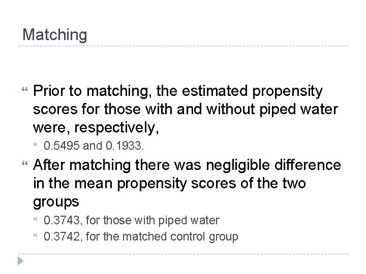
Matching Prior to matching, the estimated propensity scores for those with and without piped water were, respectively, 0. 5495 and 0. 1933. After matching there was negligible difference in the mean propensity scores of the two groups 0. 3743, for those with piped water 0. 3742, for the matched control group

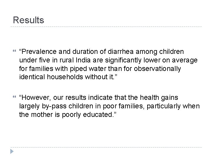
Results “Prevalence and duration of diarrhea among children under five in rural India are significantly lower on average for families with piped water than for observationally identical households without it. ” “However, our results indicate that the health gains largely by-pass children in poor families, particularly when the mother is poorly educated. ”

Conclusion Matching is a useful way to control for OBSERVABLE heterogeneity Especially when randomization or RD approach is not possible However, it requires relatively strong assumptions