Propensity Scores Alec Walker Many part of this

Propensity Scores Alec Walker Many part of this presentation were orginally created by John Seeger

“In mathematics, you don't understand things. You just get used to them. ” - John von Neumann 1903 -1957

Research Goal • Compare two treatments with respect to a health or economic outcome • “Counterfactual” ideal • If the same people had received B instead of A, how would their outcomes have differed? • What is achievable: “similar” not “same” • Comparable treatment groups • … insofar as you can tell!

Pictures for Confounding

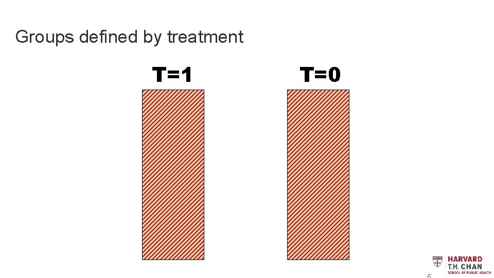
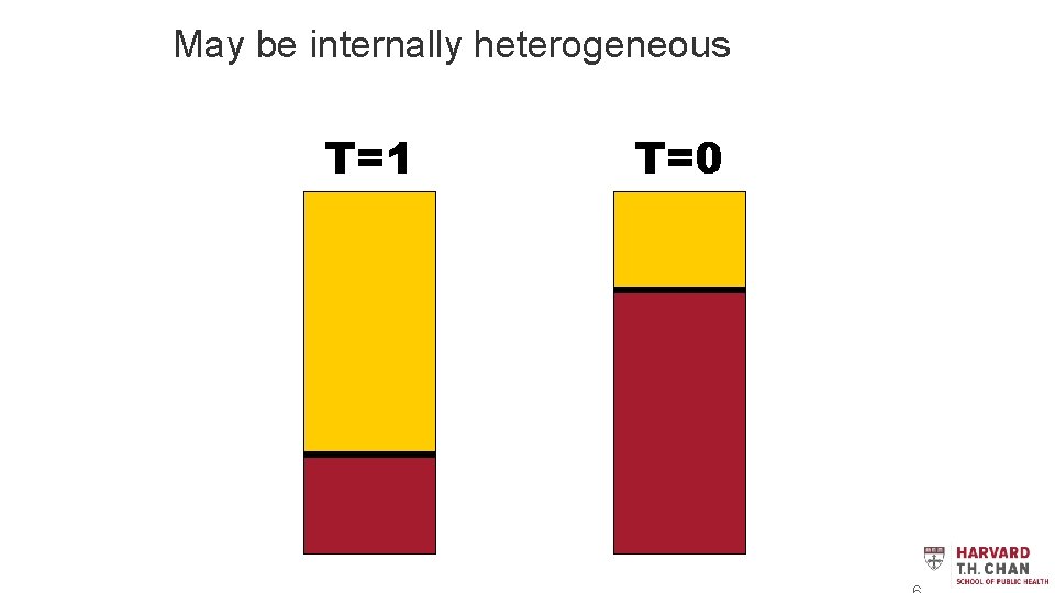
Groups defined by treatment T=1 T=0

May be internally heterogeneous T=1 T=0

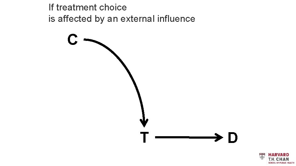
If treatment choice is affected by an external influence C T D

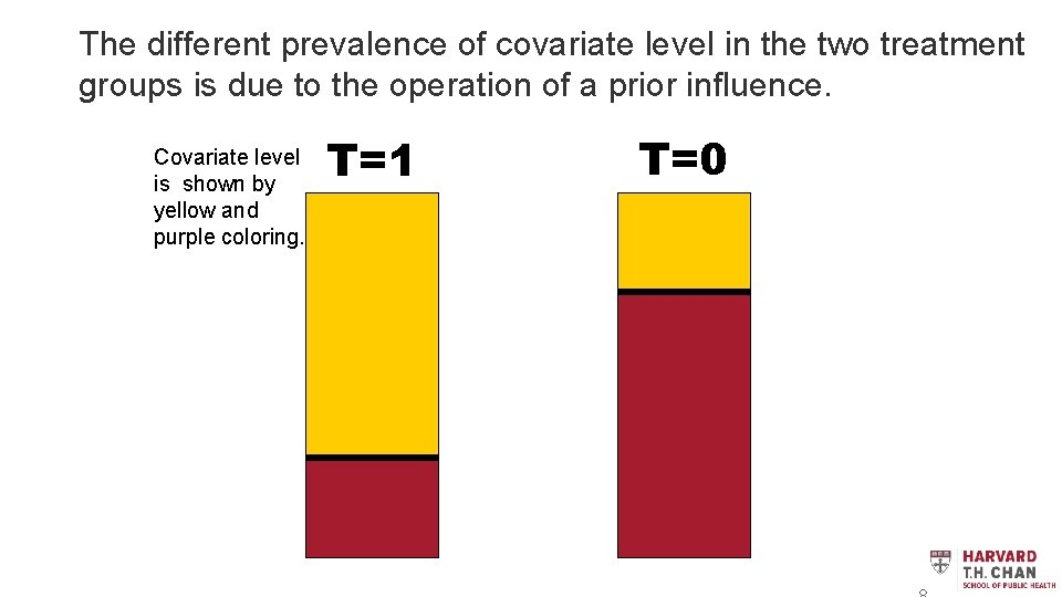
The different prevalence of covariate level in the two treatment groups is due to the operation of a prior influence. Covariate level is shown by yellow and purple coloring. T=1 T=0

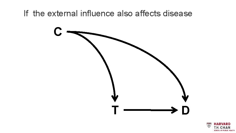
If the external influence also affects disease C T D

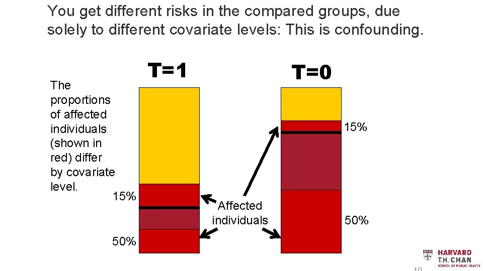
You get different risks in the compared groups, due solely to different covariate levels: This is confounding. The proportions of affected individuals (shown in red) differ by covariate level. 15% 50% T=1 T=0 15% Affected individuals 50%

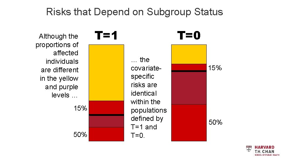
Risks that Depend on Subgroup Status Although the proportions of affected individuals are different in the yellow and purple levels … 15% 50% T=1 T=0 … the covariatespecific risks are identical within the populations defined by T=1 and T=0. 15% 50%

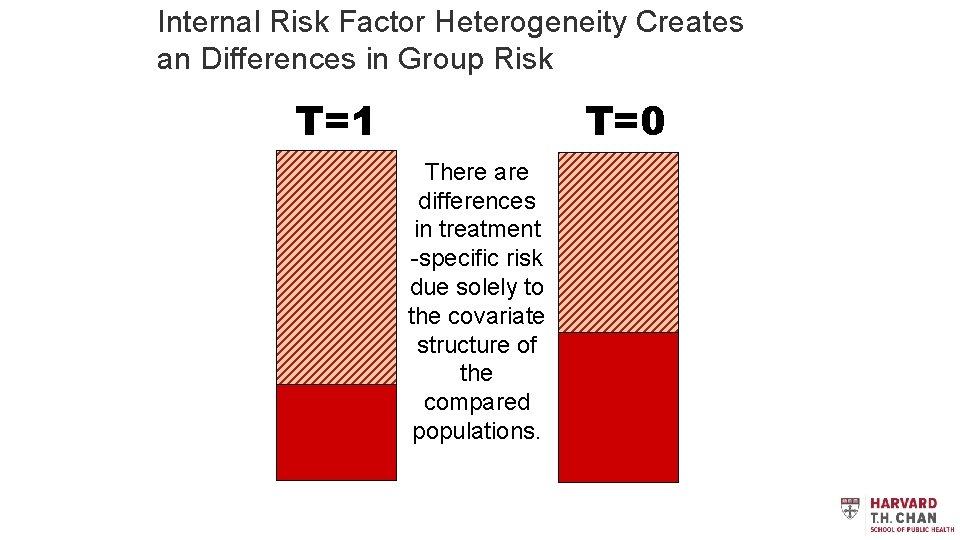
Internal Risk Factor Heterogeneity Creates an Differences in Group Risk T=1 T=0 There are differences in treatment -specific risk due solely to the covariate structure of the compared populations.

Propensity Scores to Create Populations with Similar Covariate Structure

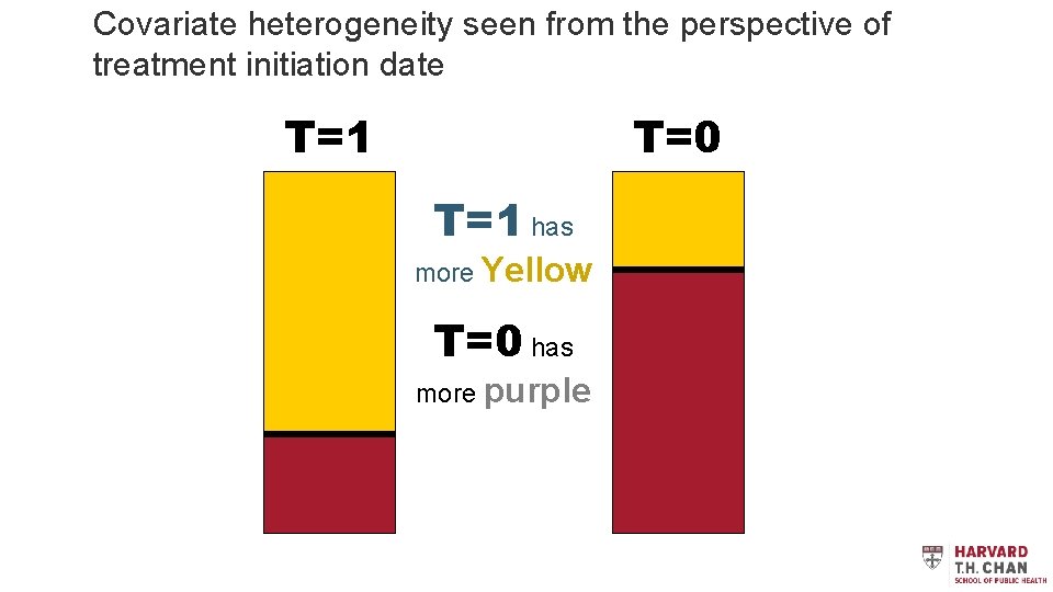
Covariate heterogeneity seen from the perspective of treatment initiation date T=1 T=0 T=1 has more Yellow T=0 has more purple

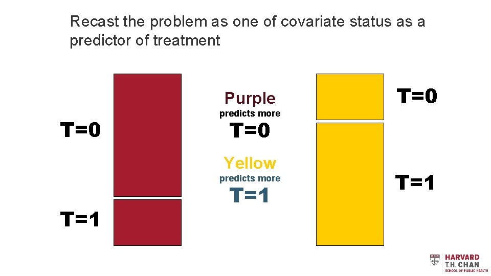
Recast the problem as one of covariate status as a predictor of treatment Purple T=0 predicts more T=0 Yellow predicts more T=1 T=0 T=1

Propensity scores • PS is the predicted probability of treatment, given all the covariates • Matching on the PS creates study populations that have balance on the covariates • Perfect for a single, dichotomous covariate • Not perfect, but very good for multiple covariates

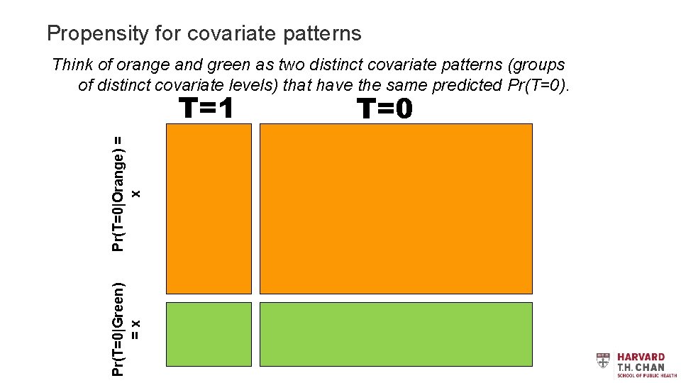
Propensity for covariate patterns Think of orange and green as two distinct covariate patterns (groups of distinct covariate levels) that have the same predicted Pr(T=0). Pr(T=0|Green) =x Pr(T=0|Orange) = x T=1 T=0

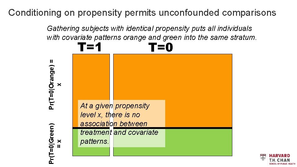
Conditioning on propensity permits unconfounded comparisons Gathering subjects with identical propensity puts all individuals with covariate patterns orange and green into the same stratum. Pr(T=0|Green) =x Pr(T=0|Orange) = x T=1 T=0 At a given propensity level x, there is no association between treatment and covariate patterns.

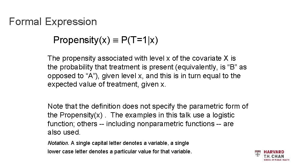
Formal Expression Propensity(x) P(T=1|x) The propensity associated with level x of the covariate X is the probability that treatment is present (equivalently, is “B” as opposed to “A”), given level x, and this is in turn equal to the expected value of treatment, given x. Note that the definition does not specify the parametric form of the Propensity(x). The examples in this talk use a logistic function; others -- including nonparametric functions -- are also used. Notation. A single capital letter denotes a variable, a single lower case letter denotes a particular value for that variable.

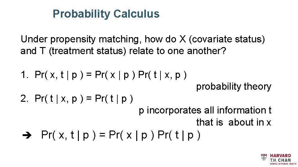
Probability Calculus Under propensity matching, how do X (covariate status) and T (treatment status) relate to one another? 1. Pr( x, t | p ) = Pr( x | p ) Pr( t | x, p ) probability theory 2. Pr( t | x, p ) = Pr( t | p ) p incorporates all information t that is about in x Pr( x, t | p ) = Pr( x | p ) Pr( t | p )

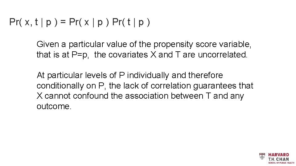
Pr( x, t | p ) = Pr( x | p ) Pr( t | p ) Given a particular value of the propensity score variable, that is at P=p, the covariates X and T are uncorrelated. At particular levels of P individually and therefore conditionally on P, the lack of correlation guarantees that X cannot confound the association between T and any outcome.

Matching on Propensity Scores

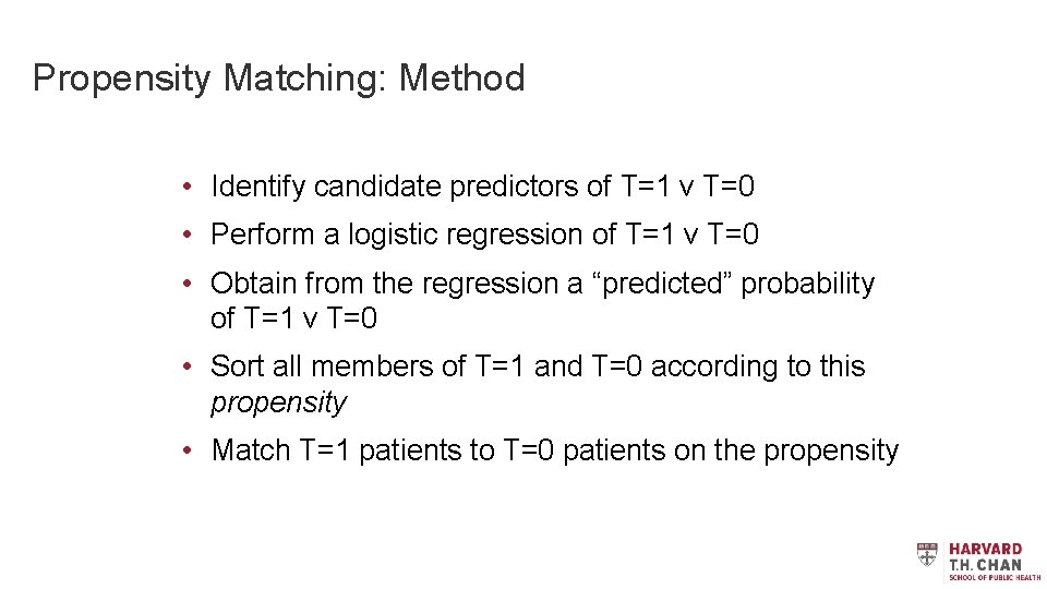
Propensity Matching: Method • Identify candidate predictors of T=1 v T=0 • Perform a logistic regression of T=1 v T=0 • Obtain from the regression a “predicted” probability of T=1 v T=0 • Sort all members of T=1 and T=0 according to this propensity • Match T=1 patients to T=0 patients on the propensity

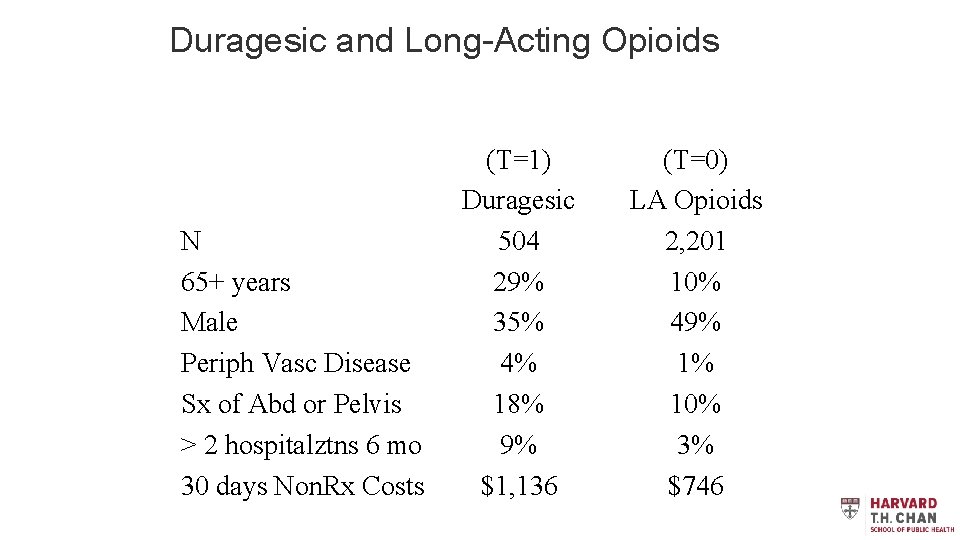
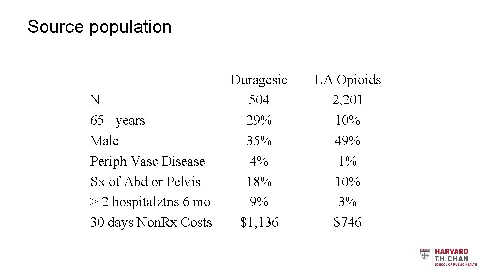
Duragesic and Long-Acting Opioids N 65+ years Male Periph Vasc Disease Sx of Abd or Pelvis > 2 hospitalztns 6 mo 30 days Non. Rx Costs (T=1) Duragesic 504 29% 35% 4% 18% 9% $1, 136 (T=0) LA Opioids 2, 201 10% 49% 1% 10% 3% $746

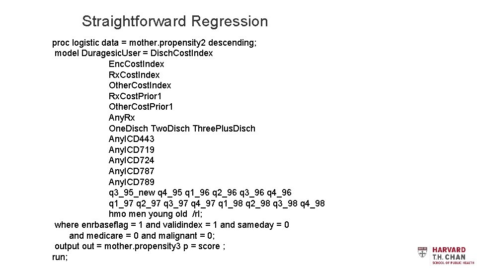
Straightforward Regression proc logistic data = mother. propensity 2 descending; model Duragesic. User = Disch. Cost. Index Enc. Cost. Index Rx. Cost. Index Other. Cost. Index Rx. Cost. Prior 1 Other. Cost. Prior 1 Any. Rx One. Disch Two. Disch Three. Plus. Disch Any. ICD 443 Any. ICD 719 Any. ICD 724 Any. ICD 787 Any. ICD 789 q 3_95_new q 4_95 q 1_96 q 2_96 q 3_96 q 4_96 q 1_97 q 2_97 q 3_97 q 4_97 q 1_98 q 2_98 q 3_98 q 4_98 hmo men young old /rl; where enrbaseflag = 1 and validindex = 1 and sameday = 0 and medicare = 0 and malignant = 0; output out = mother. propensity 3 p = score ; run;

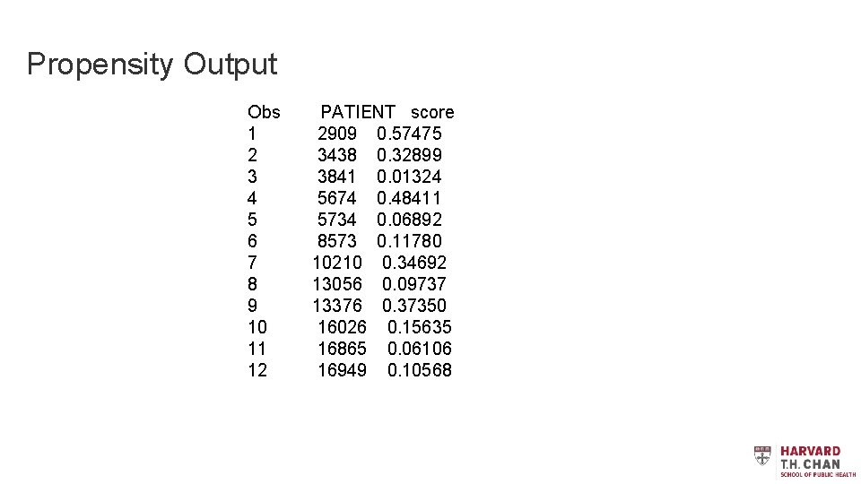
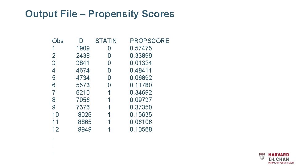
Propensity Output Obs PATIENT score 1 2909 0. 57475 2 3438 0. 32899 3 3841 0. 01324 4 5674 0. 48411 5 5734 0. 06892 6 8573 0. 11780 7 10210 0. 34692 8 13056 0. 09737 9 13376 0. 37350 10 16026 0. 15635 11 16865 0. 06106 12 16949 0. 10568

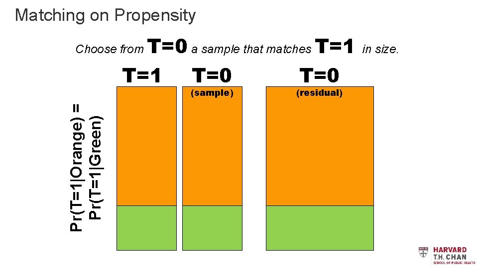
Matching on Propensity T=0 a sample that matches T=1 T=0 Choose from Pr(T=1|Orange) = Pr(T=1|Green) (sample) (residual) in size.

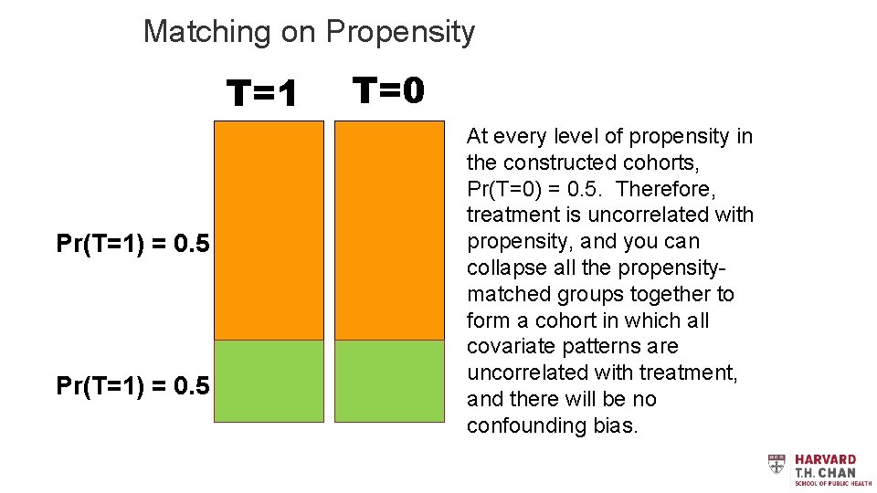
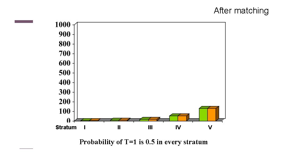
Matching on Propensity T=1 Pr(T=1) = 0. 5 T=0 At every level of propensity in the constructed cohorts, Pr(T=0) = 0. 5. Therefore, treatment is uncorrelated with propensity, and you can collapse all the propensitymatched groups together to form a cohort in which all covariate patterns are uncorrelated with treatment, and there will be no confounding bias.

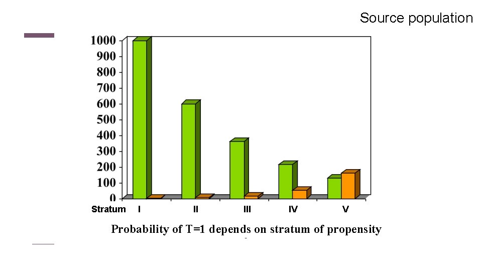
Source population Stratum I II IV V Probability of T=1 depends on stratum of propensity

After matching Stratum I II IV Probability of T=1 is 0. 5 in every stratum V

Source population N 65+ years Male Periph Vasc Disease Sx of Abd or Pelvis > 2 hospitalztns 6 mo 30 days Non. Rx Costs Duragesic 504 29% 35% 4% 18% 9% $1, 136 LA Opioids 2, 201 10% 49% 1% 10% 3% $746

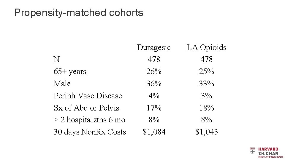
Propensity-matched cohorts N 65+ years Male Periph Vasc Disease Sx of Abd or Pelvis > 2 hospitalztns 6 mo 30 days Non. Rx Costs Duragesic 478 26% 36% 4% 17% 8% $1, 084 LA Opioids 478 25% 33% 3% 18% 8% $1, 043

Example – Propensity matching to undo the confounding by indication in a comparative effectiveness study

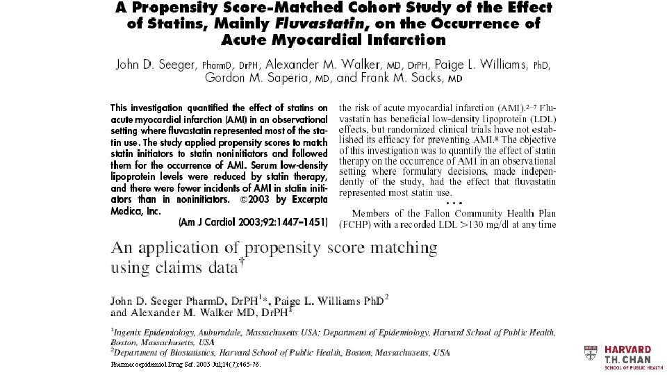
Pharmacoepidemiol Drug Saf. 2005 Jul; 14(7): 465 -76.

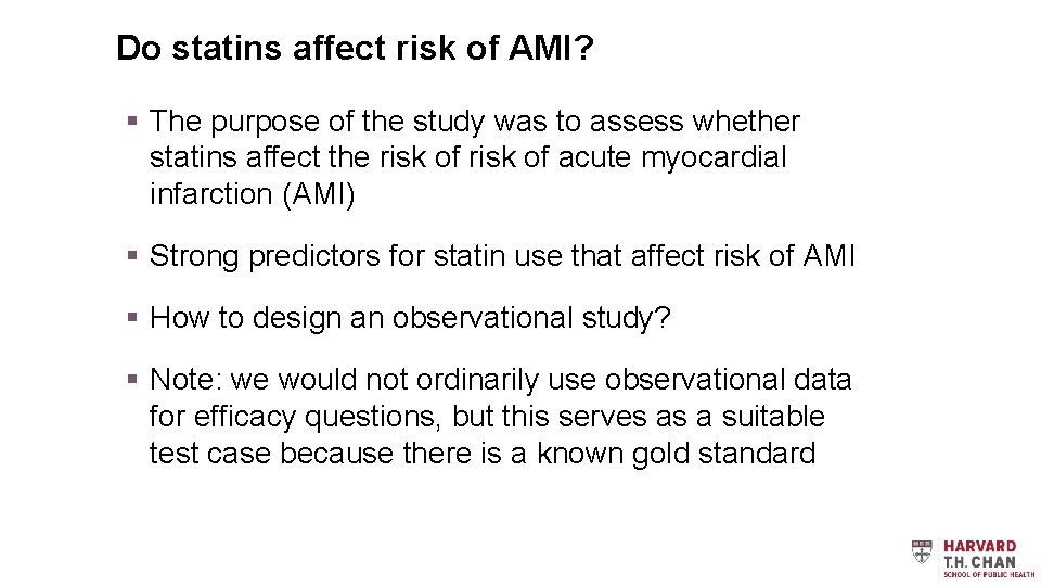
Do statins affect risk of AMI? § The purpose of the study was to assess whether statins affect the risk of acute myocardial infarction (AMI) § Strong predictors for statin use that affect risk of AMI § How to design an observational study? § Note: we would not ordinarily use observational data for efficacy questions, but this serves as a suitable test case because there is a known gold standard

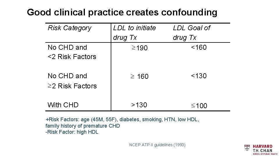
Good clinical practice creates confounding Risk Category No CHD and <2 Risk Factors No CHD and ³ 2 Risk Factors With CHD LDL to initiate drug Tx ³ 190 LDL Goal of drug Tx <160 ³ 160 <130 >130 £ 100 +Risk Factors: age (45 M, 55 F), diabetes, smoking, HTN, low HDL, family history of premature CHD -Risk Factor: high HDL NCEP ATP II guidelines (1993)

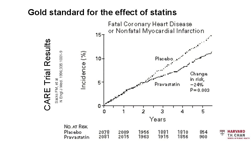
Sacks FM, et al N Engl J Med. 1996; 335: 1001 -9 CARE Trial Results Gold standard for the effect of statins

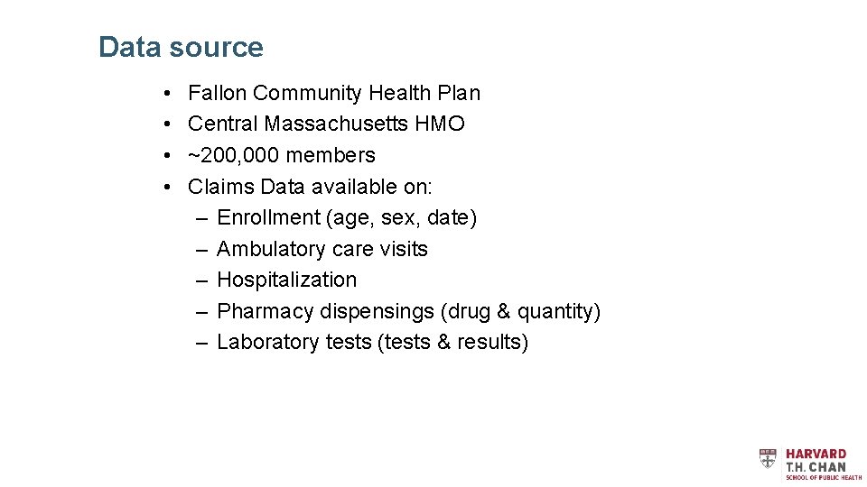
Data source • • Fallon Community Health Plan Central Massachusetts HMO ~200, 000 members Claims Data available on: – Enrollment (age, sex, date) – Ambulatory care visits – Hospitalization – Pharmacy dispensings (drug & quantity) – Laboratory tests (tests & results)

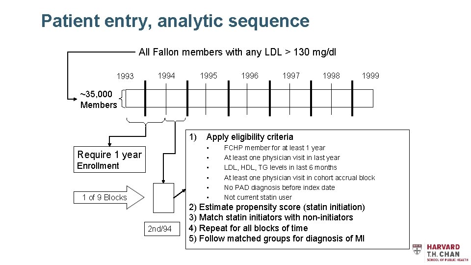
Patient entry, analytic sequence All Fallon members with any LDL > 130 mg/dl 1993 1994 1995 1996 1997 1998 1999 ~35, 000 Members 1) Apply eligibility criteria • • • Require 1 year Enrollment 1 of 9 Blocks 2 nd/94 FCHP member for at least 1 year At least one physician visit in last year LDL, HDL, TG levels in last 6 months At least one physician visit in cohort accrual block No PAD diagnosis before index date Not current statin user 2) Estimate propensity score (statin initiation) 3) Match statin initiators with non-initiators 4) Repeat for all blocks of time 5) Follow matched groups for diagnosis of MI

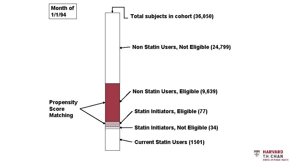
Month of 1/1/94 Total subjects in cohort (36, 050) Non Statin Users, Not Eligible (24, 799) Non Statin Users, Eligible (9, 639) Propensity Score Matching Statin Initiators, Eligible (77) Statin Initiators, Not Eligible (34) Current Statin Users (1501)

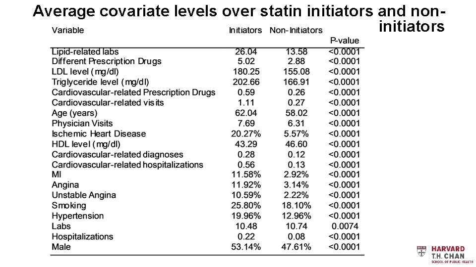
Average covariate levels over statin initiators and noninitiators

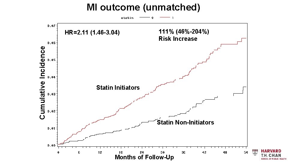
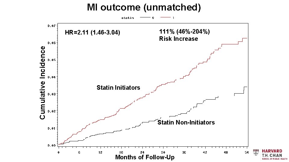
MI outcome (unmatched) Cumulative Incidence HR=2. 11 (1. 46 -3. 04) 111% (46%-204%) Risk Increase Statin Initiators Statin Non-Initiators Months of Follow-Up

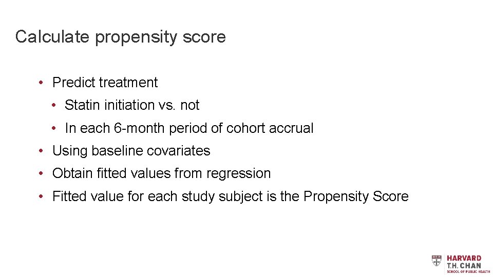
Calculate propensity score • Predict treatment • Statin initiation vs. not • In each 6 -month period of cohort accrual • Using baseline covariates • Obtain fitted values from regression • Fitted value for each study subject is the Propensity Score

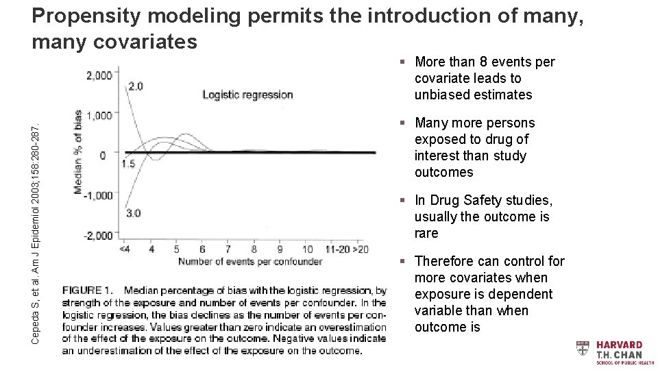
Propensity modeling permits the introduction of many, Construct Rich Model many covariates Cepeda S, et al. Am J Epidemiol 2003; 158: 280 -287. § More than 8 events per covariate leads to unbiased estimates § Many more persons exposed to drug of interest than study outcomes § In Drug Safety studies, usually the outcome is rare § Therefore can control for more covariates when exposure is dependent variable than when outcome is

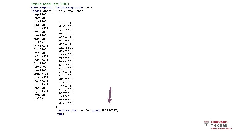
*build model for 9501; proc logistic descending data=new 1; model statin = male smok obes age 9501 ang 9501 usa 9501 ins 9501 chf 9501 diab 9501 isch 9501 skca 9501 ath 9501 depr 9501 cva 9501 adj 9501 usa 9501 schz 9501 mi 9501 deb 9501 olmi 9501 rheu 9501 htn 9501 days 9501 tia 9501 lres 9501 afib 9501 tres 9501 ascv 9501 hres 9501 hth 9501 hbac 9501 ost 9501 cvhp 9501 cvs 9501 ekg 9501 htdx 9501 cvrx 9501 circ 9501 cvvs 9501 cond 9501 llab 9501 rvsc 9501 lab 9501 hhd 9501 cvdg 9501 dysr 9501 hosp 9501 hrt 9501 rx 9501 ns 9501 vist 9501 diag 9501 ; output out=psmodel pred=PROPSCORE; run;

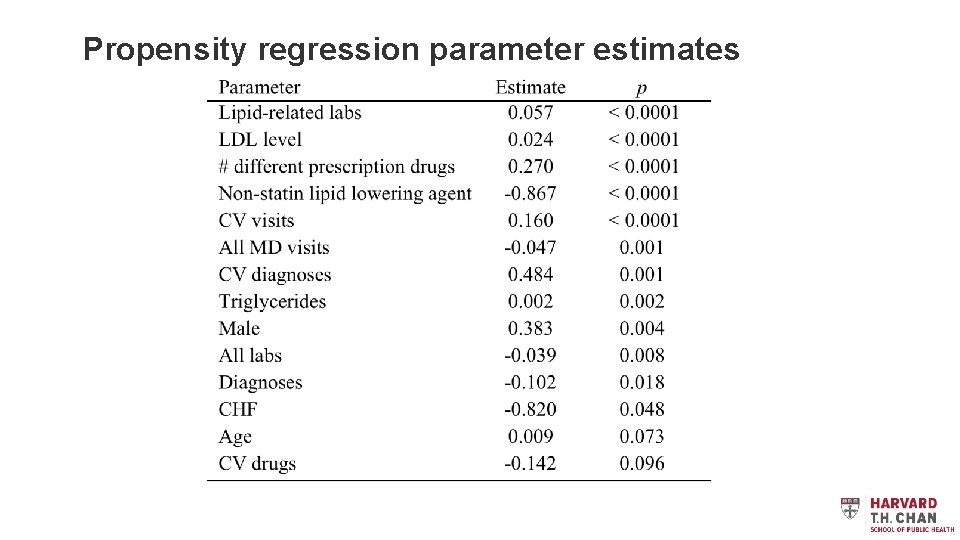
Propensity regression parameter estimates

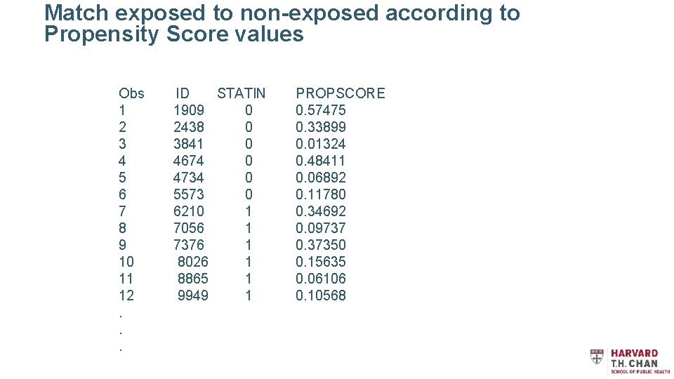
Output File – Propensity Scores Obs ID STATIN 1 1909 0 2 2438 0 3 3841 0 4 4674 0 5 4734 0 6 5573 0 7 6210 1 8 7056 1 9 7376 1 10 8026 1 11 8865 1 12 9949 1. . . PROPSCORE 0. 57475 0. 33899 0. 01324 0. 48411 0. 06892 0. 11780 0. 34692 0. 09737 0. 37350 0. 15635 0. 06106 0. 10568

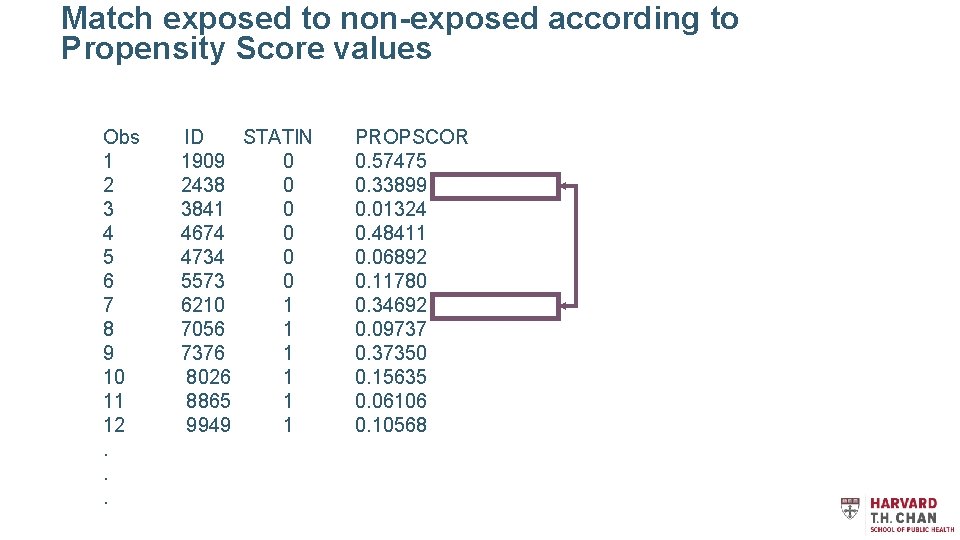
Match exposed to non-exposed according to Propensity Score values Obs ID STATIN 1 1909 0 2 2438 0 3 3841 0 4 4674 0 5 4734 0 6 5573 0 7 6210 1 8 7056 1 9 7376 1 10 8026 1 11 8865 1 12 9949 1. . . PROPSCORE 0. 57475 0. 33899 0. 01324 0. 48411 0. 06892 0. 11780 0. 34692 0. 09737 0. 37350 0. 15635 0. 06106 0. 10568

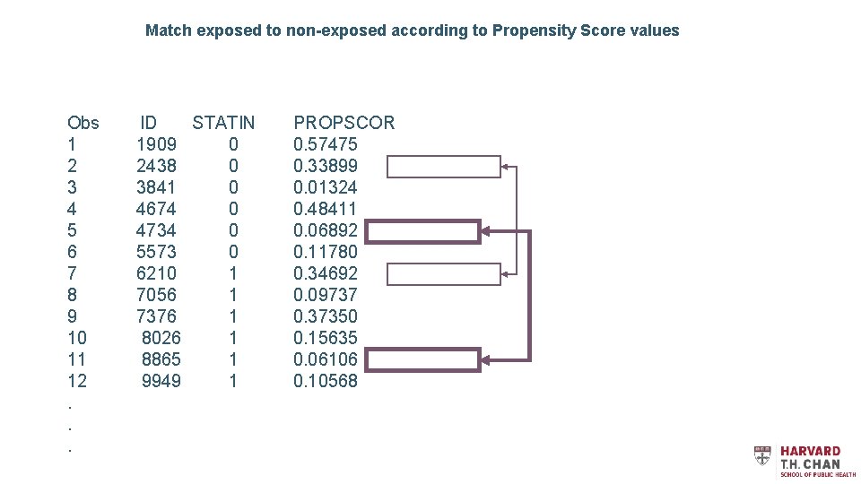
Match exposed to non-exposed according to Propensity Score values Obs ID STATIN 1 1909 0 2 2438 0 3 3841 0 4 4674 0 5 4734 0 6 5573 0 7 6210 1 8 7056 1 9 7376 1 10 8026 1 11 8865 1 12 9949 1. . . PROPSCOR 0. 57475 0. 33899 0. 01324 0. 48411 0. 06892 0. 11780 0. 34692 0. 09737 0. 37350 0. 15635 0. 06106 0. 10568

Match exposed to non-exposed according to Propensity Score values Obs ID STATIN 1 1909 0 2 2438 0 3 3841 0 4 4674 0 5 4734 0 6 5573 0 7 6210 1 8 7056 1 9 7376 1 10 8026 1 11 8865 1 12 9949 1. . . PROPSCOR 0. 57475 0. 33899 0. 01324 0. 48411 0. 06892 0. 11780 0. 34692 0. 09737 0. 37350 0. 15635 0. 06106 0. 10568

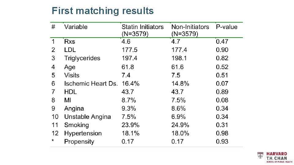
Balance achieved by matching Only 1 of 52 variables sig. different at P<0. 05

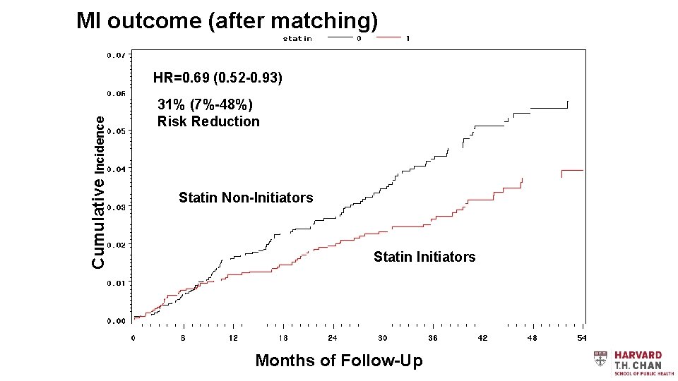
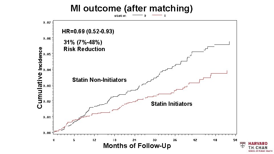
MI outcome (after matching) Cumulative Incidence HR=0. 69 (0. 52 -0. 93) 31% (7%-48%) Risk Reduction Statin Non-Initiators Statin Initiators Months of Follow-Up

Interpreting Propensity Coefficients

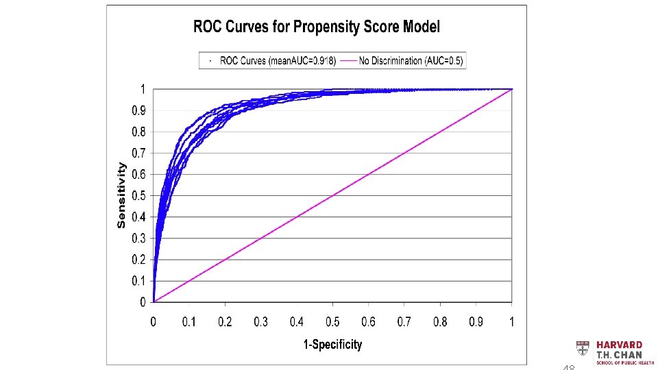
When Is the Model Sufficient?

First matching results

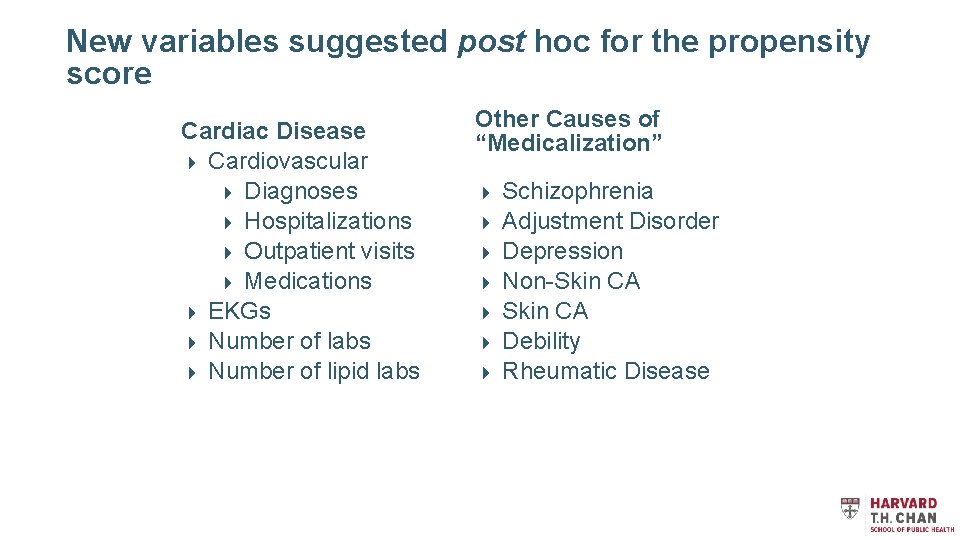
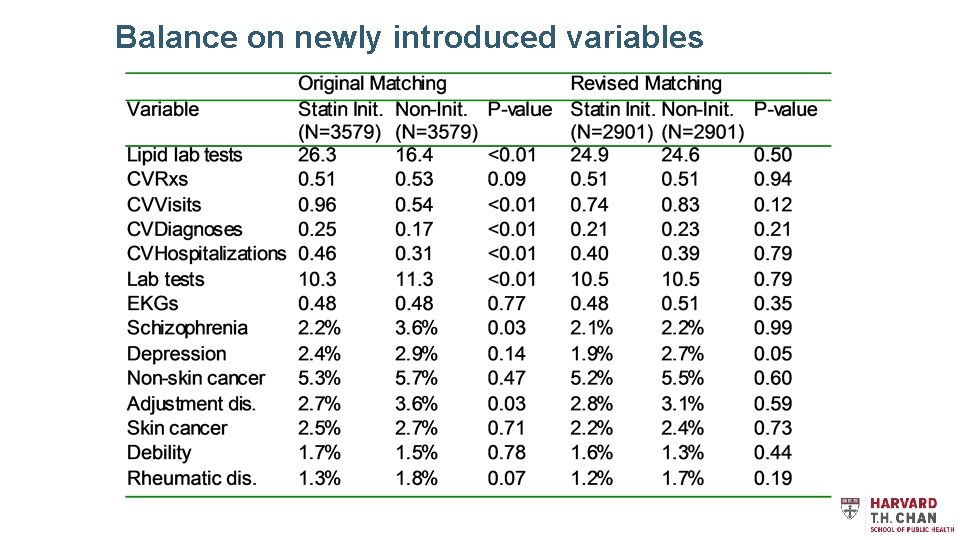
New variables suggested post hoc for the propensity score Cardiac Disease 4 Cardiovascular 4 Diagnoses 4 Hospitalizations 4 Outpatient visits 4 Medications 4 EKGs 4 Number of labs 4 Number of lipid labs Other Causes of “Medicalization” 4 4 4 4 Schizophrenia Adjustment Disorder Depression Non-Skin CA Debility Rheumatic Disease

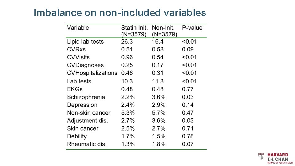
Imbalance on non-included variables

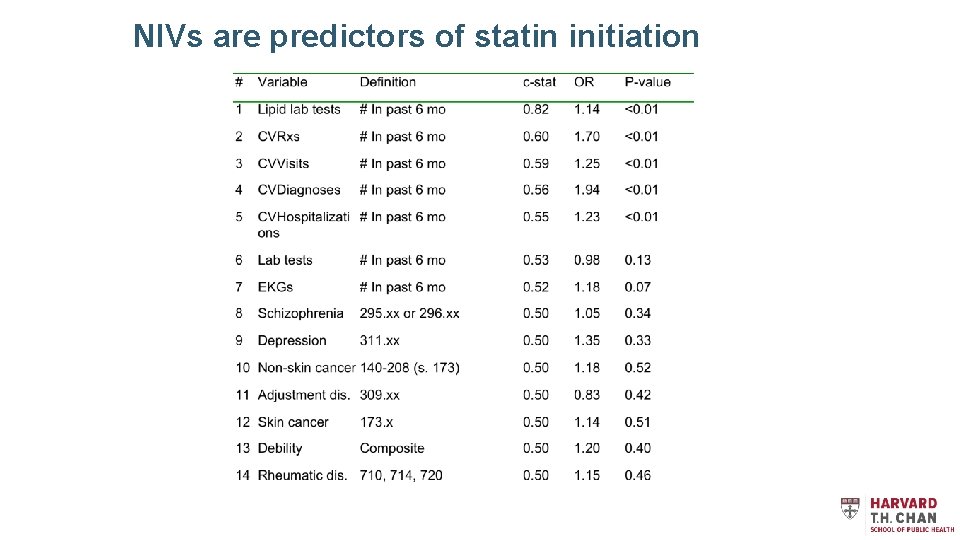
NIVs are predictors of statin initiation

New ranking of predictors

Balance on newly introduced variables

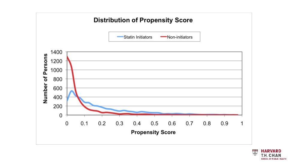
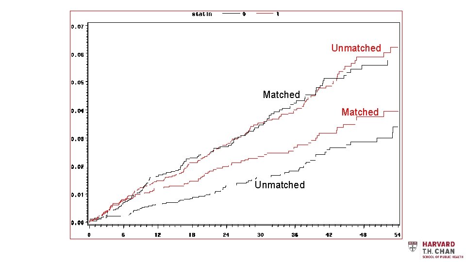
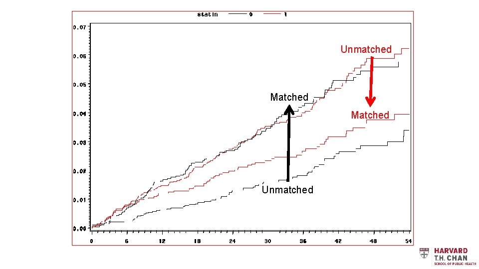
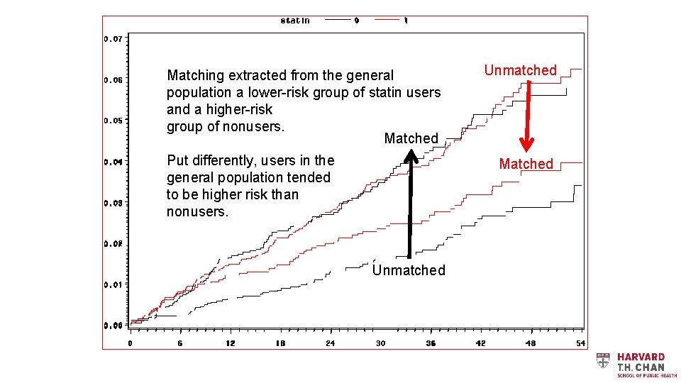
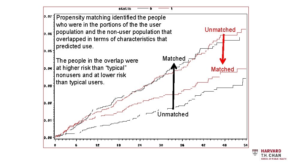
The populations selected are a special case – the region of overlap of preferences

MI outcome (unmatched) Cumulative Incidence HR=2. 11 (1. 46 -3. 04) 111% (46%-204%) Risk Increase Statin Initiators Statin Non-Initiators Months of Follow-Up

MI outcome (after matching) Cumulative Incidence HR=0. 69 (0. 52 -0. 93) 31% (7%-48%) Risk Reduction Statin Non-Initiators Statin Initiators Months of Follow-Up

Unmatched Matched Unmatched

Unmatched Matched Unmatched

Matching extracted from the general population a lower-risk group of statin users and a higher-risk group of nonusers. Matched Put differently, users in the general population tended to be higher risk than nonusers. Unmatched Matched Unmatched

Propensity matching identified the people who were in the portions of the user population and the non-user population that overlapped in terms of characteristics that predicted use. The people in the overlap were at higher risk than “typical” nonusers and at lower risk than typical users. Unmatched Matched Unmatched

Thank You! Copyright © President and Fellows of Harvard College

Thank You! Copyright © President and Fellows of Harvard College