Peter J Russell CHAPTER 23 Quantitative Genetics edited

Peter J. Russell CHAPTER 23 Quantitative Genetics edited by Yue-Wen Wang Ph. D. Dept. of Agronomy, 台大農藝系 NTU 遺傳學 601 20000 1

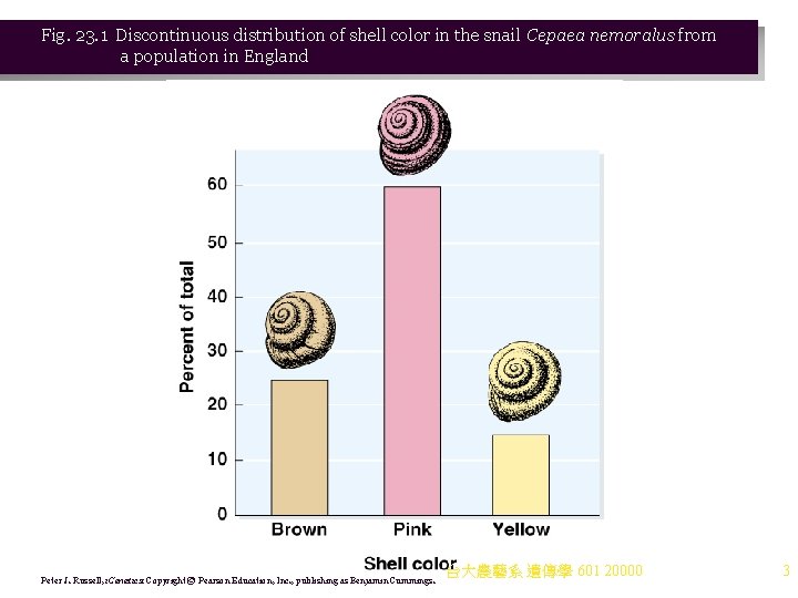
1. Traits with a few distinct phenotypes are discontinuous traits. There is usually a simple relationship between the genes responsible and formation of the phenotype. 2. Often, penetrance, expressivity, pleiotropy, epistasis and environmental factors are involved in producing a continuous distribution of phenotypes (continuous traits). Quantitative genetics is used to characterize continuous traits. 台大農藝系 遺傳學 601 20000 2

Fig. 23. 1 Discontinuous distribution of shell color in the snail Cepaea nemoralus from a population in England Peter J. Russell, i. Genetics: Copyright © Pearson Education, Inc. , publishing as Benjamin Cummings. 台大農藝系 遺傳學 601 20000 3

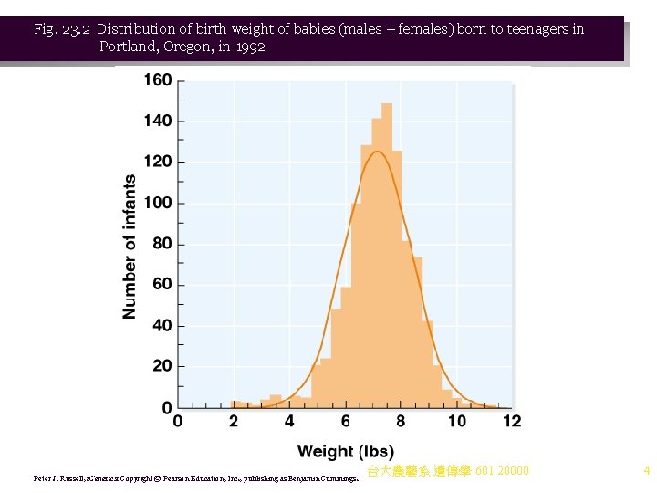
Fig. 23. 2 Distribution of birth weight of babies (males + females) born to teenagers in Portland, Oregon, in 1992 Peter J. Russell, i. Genetics: Copyright © Pearson Education, Inc. , publishing as Benjamin Cummings. 台大農藝系 遺傳學 601 20000 4

The Nature of Continuous Traits 1. Statistical study of continuous traits began with human traits such as height, weight and mental traits, even before Mendel’s principles were understood. 2. Galton and Pearson (late 1800 s) showed that these traits are statistically linked between parents and offspring, but could not determine the mode of transmission. 3. Johannsen (1903) showed that continuous variation in bean seed weight is partly genetic and partly environmental. 4. Nilsson-Ehle proposed that continuous variation in wheat results from multiple genes segregating by Mendelian principles. 5. Fisher demonstrated that mathematical models of Mendelian and population genetics also apply to traits controlled by multiple gene loci. 台大農藝系 遺傳學 601 20000 5

Why Some Traits Have Continuous Phenotypes 1. Multiple traits arise in several ways: a. When a trait is influenced by many loci (polygenic), a range of phenotypes results from the numerous genotypes. For example: i. When a single locus with two alleles determines a trait, there are three possible genotypes (AA, Aa and aa). ii. With two loci, each with two alleles, there are nine possible genotypes. iii. In general, the number of genotypes is 3 n, where n is the number of loci with two alleles. If the number of alleles is higher, the number of genotypes will be even larger. iv. If every genotype in a polygenic trait produces a different phenotype and the differences between phenotypes are slight, the trait appears to be continuous. v. More often, several genotypes produce the same phenotype for a polygenic trait. Reasons for this include: (1) Dominance, producing the same phenotype in both heterozygous and homozygous dominant individuals. (2) Epistasis, resulting from control of the expression of other loci. 台大農藝系 遺傳學 601 20000 6

2. A range of phenotypes is also produced when environmental factors affect the trait. Each genotype will have a range of possible phenotypes, the norm of reaction. 3. Most traits are influenced by both multiple genotypes and environmental factors, and are thus multifactorial. The rules of transmission genetics and gene function still apply. Understanding the role of each gene is difficult, and so quantitative genetics is employed to analyze continuous traits. 台大農藝系 遺傳學 601 20000 7

Questions Studied in Quantitative Genetics 1. What role is played by genetics, and what role by environment? 2. How many genes are involved in producing phenotypes of the trait? 3. Do some genes play a major role in determining phenotype, while others modify it only slightly, or are the contributions equal? 4. Do the alleles interact with each other to produce additive effects? 5. What changes occur when there is selection for a phenotype, and do other traits also change? 6. What method of selecting and mating individuals will produce desired phenotypes in the progeny? 台大農藝系 遺傳學 601 20000 8

Statistical Tools 1. Genes are always expressed in an environmental context, and without genes there would be nothing to express. The nature vs. nurture question provides an opportunity to examine the relative contributions of both. 2. How much of a variation in phenotype (VP) is due to genetic variation (VG) and how much to environmental variation (VE)? This can be expressed: VP = VG + VE. 3. To work this equation, variation must be measured and then partitioned into genetic and environmental components. 台大農藝系 遺傳學 601 20000 9

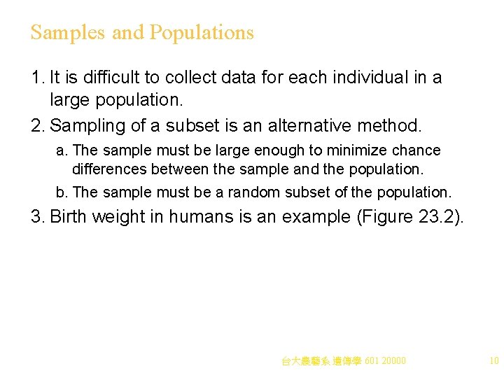
Samples and Populations 1. It is difficult to collect data for each individual in a large population. 2. Sampling of a subset is an alternative method. a. The sample must be large enough to minimize chance differences between the sample and the population. b. The sample must be a random subset of the population. 3. Birth weight in humans is an example (Figure 23. 2). 台大農藝系 遺傳學 601 20000 10

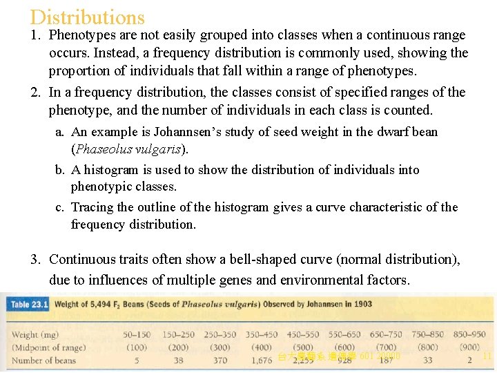
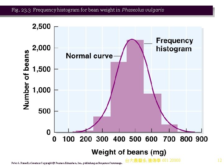
Distributions 1. Phenotypes are not easily grouped into classes when a continuous range occurs. Instead, a frequency distribution is commonly used, showing the proportion of individuals that fall within a range of phenotypes. 2. In a frequency distribution, the classes consist of specified ranges of the phenotype, and the number of individuals in each class is counted. a. An example is Johannsen’s study of seed weight in the dwarf bean (Phaseolus vulgaris). b. A histogram is used to show the distribution of individuals into phenotypic classes. c. Tracing the outline of the histogram gives a curve characteristic of the frequency distribution. 3. Continuous traits often show a bell-shaped curve (normal distribution), due to influences of multiple genes and environmental factors. 台大農藝系 遺傳學 601 20000 11

Fig. 23. 3 Frequency histogram for bean weight in Phaseolus vulgaris Peter J. Russell, i. Genetics: Copyright © Pearson Education, Inc. , publishing as Benjamin Cummings. 台大農藝系 遺傳學 601 20000 12

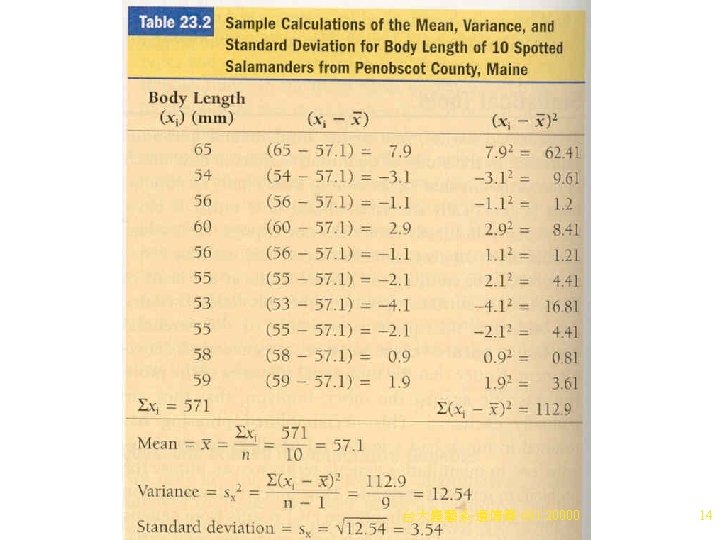
The Mean 1. Frequency distribution of a phenotypic trait can be summarized with two statistics, the mean and the variance. 2. The mean (average) represents the center of the phenotype distribution, and is calculated simply by adding all individual measurements and then dividing by the number of measurements added. 3. An example is body length of spotted salamanders (Table 23. 2). 4. Another example is East’s study of tobacco flower length in genetic crosses. a. He crossed a short-flowered strain (mean length of 40. 4 mm) with a long-flowered strain (mean length of 93. 1 mm). b. The F 1 progeny (173 plants) had a mean flower length of 63. 5 mm. 台大農藝系 遺傳學 601 20000 13

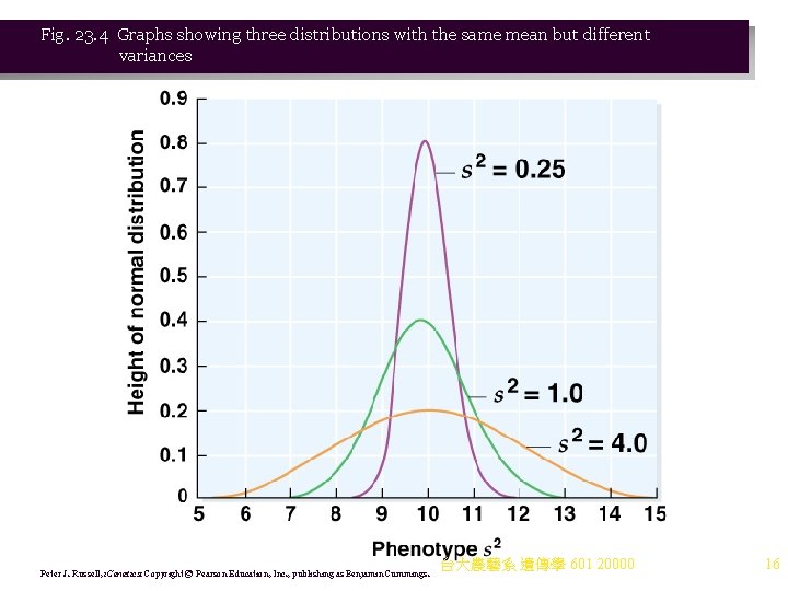
The Variance and the Standard Deviation 1. Variance is the measure of how much the individual measurements spread out around the mean (how variable they are). a. Two sets of measurements may have the same mean, but different variances (Figure 23. 4). b. The variance (s 2) is the average squared deviation from the mean. To calculate s 2: i. Subtract the mean from each individual measurement. ii. Square the difference for each. iii. Add the squared values. iv. Divide by the number of original measurements minus 1 (n - 1). c. Standard deviation is used more often than variance, because it shares the same units as the original measurements (rather than units 2 as in variance). Standard deviation is the square root of the variance. d. Table 23. 2 shows sample calculations for variance and standard deviation. i. A broad curve indicates a large variability in the measurements and a large standard deviation. ii. A narrow curve implies little variability and a遺傳學 small 601 standard deviation. 台大農藝系 20000 15

Fig. 23. 4 Graphs showing three distributions with the same mean but different variances Peter J. Russell, i. Genetics: Copyright © Pearson Education, Inc. , publishing as Benjamin Cummings. 台大農藝系 遺傳學 601 20000 16

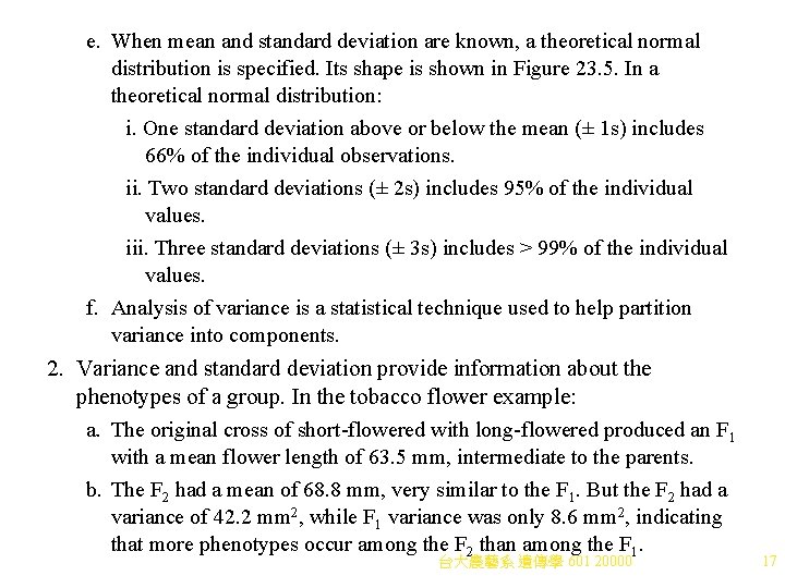
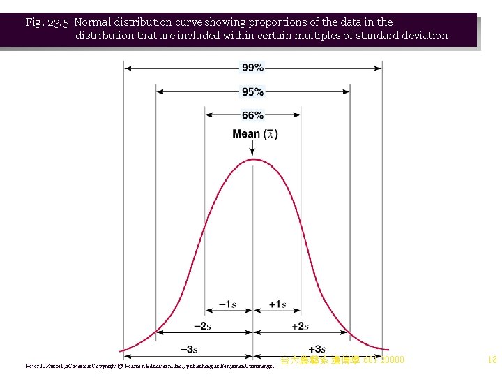
e. When mean and standard deviation are known, a theoretical normal distribution is specified. Its shape is shown in Figure 23. 5. In a theoretical normal distribution: i. One standard deviation above or below the mean (± 1 s) includes 66% of the individual observations. ii. Two standard deviations (± 2 s) includes 95% of the individual values. iii. Three standard deviations (± 3 s) includes > 99% of the individual values. f. Analysis of variance is a statistical technique used to help partition variance into components. 2. Variance and standard deviation provide information about the phenotypes of a group. In the tobacco flower example: a. The original cross of short-flowered with long-flowered produced an F 1 with a mean flower length of 63. 5 mm, intermediate to the parents. b. The F 2 had a mean of 68. 8 mm, very similar to the F 1. But the F 2 had a variance of 42. 2 mm 2, while F 1 variance was only 8. 6 mm 2, indicating that more phenotypes occur among the F 2 than among the F 1. 台大農藝系 遺傳學 601 20000 17

Fig. 23. 5 Normal distribution curve showing proportions of the data in the distribution that are included within certain multiples of standard deviation Peter J. Russell, i. Genetics: Copyright © Pearson Education, Inc. , publishing as Benjamin Cummings. 台大農藝系 遺傳學 601 20000 18

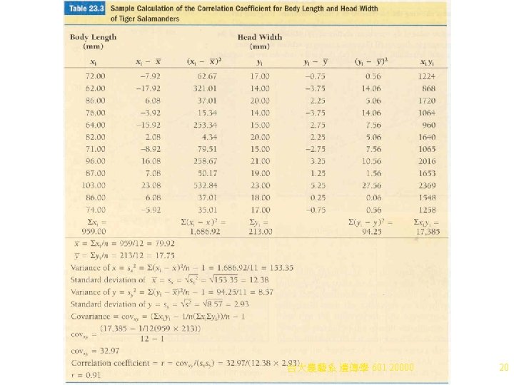
Correlation 1. Traits in individuals are often correlated, due to the pleiotropic effects of genes and environmental factors. Height and weight, for example, are aspects of a more general trait size. a. When traits are correlated, change in one is associated with change in the other (e. g. , human leg and arm length are usually correlated). i. Correlation coefficient measures the strength of association between two variables in the same individual or experimental unit. In the arm and leg example, x = arm length, and y = leg length: (1) Obtain the covariance of x and y (the variance shared by both traits) by taking the deviation from the mean for each. (2) Take the product of each pair of x and y values. (3) Add all products together. (4) Divide the sum by n - 1 to give the covariance of x and y where n= the number of xy pairs. (5) The correlation coefficient (r) is then obtained by dividing the covariance by the product of the standard deviations of x and y (Table 23. 3). 台大農藝系 遺傳學 601 20000 19

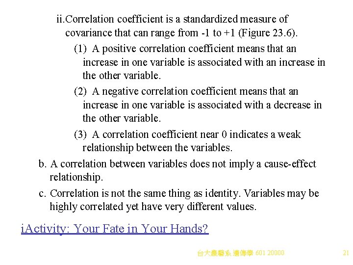
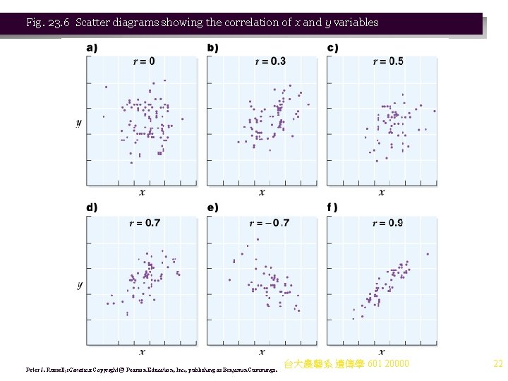
ii. Correlation coefficient is a standardized measure of covariance that can range from -1 to +1 (Figure 23. 6). (1) A positive correlation coefficient means that an increase in one variable is associated with an increase in the other variable. (2) A negative correlation coefficient means that an increase in one variable is associated with a decrease in the other variable. (3) A correlation coefficient near 0 indicates a weak relationship between the variables. b. A correlation between variables does not imply a cause-effect relationship. c. Correlation is not the same thing as identity. Variables may be highly correlated yet have very different values. i. Activity: Your Fate in Your Hands? 台大農藝系 遺傳學 601 20000 21

Fig. 23. 6 Scatter diagrams showing the correlation of x and y variables Peter J. Russell, i. Genetics: Copyright © Pearson Education, Inc. , publishing as Benjamin Cummings. 台大農藝系 遺傳學 601 20000 22

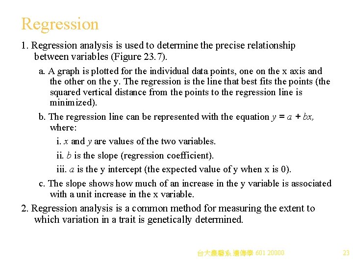
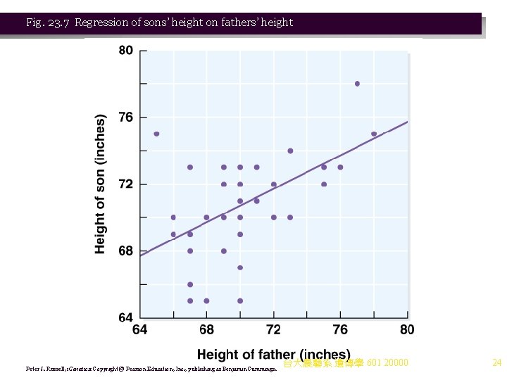
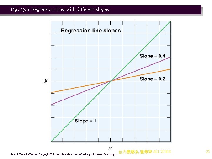
Regression 1. Regression analysis is used to determine the precise relationship between variables (Figure 23. 7). a. A graph is plotted for the individual data points, one on the x axis and the other on the y. The regression is the line that best fits the points (the squared vertical distance from the points to the regression line is minimized). b. The regression line can be represented with the equation y = a + bx, where: i. x and y are values of the two variables. ii. b is the slope (regression coefficient). iii. a is the y intercept (the expected value of y when x is 0). c. The slope shows how much of an increase in the y variable is associated with a unit increase in the x variable. 2. Regression analysis is a common method for measuring the extent to which variation in a trait is genetically determined. 台大農藝系 遺傳學 601 20000 23

Fig. 23. 7 Regression of sons’ height on fathers’ height Peter J. Russell, i. Genetics: Copyright © Pearson Education, Inc. , publishing as Benjamin Cummings. 台大農藝系 遺傳學 601 20000 24

Fig. 23. 8 Regression lines with different slopes Peter J. Russell, i. Genetics: Copyright © Pearson Education, Inc. , publishing as Benjamin Cummings. 台大農藝系 遺傳學 601 20000 25

Analysis of Variance 1. Analysis of variance (ANOVA) determines if differences in means are significant, and divides the variance into components. a. It can tell whether a variation between two groups is likely to be due to chance, rather than to a true difference. b. ANOVA can also determine how much of a difference is due to a factor like genetics or the environment, by partitioning the variance. 2. Details of the calculations are beyond the scope of this text. 台大農藝系 遺傳學 601 20000 26

Polygenic Inheritance 1. In the experiments described here, it was not clear at first how these traits were inherited, only that their pattern of inheritance differed from that seen with discontinuous traits. 台大農藝系 遺傳學 601 20000 27

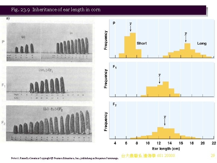
Inheritance of Ear Length in Corn 1. Emerson and East (1913) experimented with two pure-breeding strains of corn. a. Each strain shows little variation in ear length. i. The Black Mexican sweet corn variety has short ears (mean length 6. 63 cm) with a standard deviation (s) of 0. 816. ii. Tom Thumb popcorn has long ears (mean length 16. 80 cm), and s = 1. 887. b. The two strains were crossed, and the F 1 plants interbred (Figure 23. 9). i. The mean ear length in the F 1 is 12. 12 cm, approximately intermediate, and s = 1. 519. ii. Since both parents were true-breeding, all F 1 plants should have the same heterozygous genotype, and any variation in length would be due to environmental factors. iii. The mean ear length of the F 2 is 12. 89 cm, very similar to the F 1, but in the F 2, s = 2. 252, reflecting its greater variability. iv. It is expected that the environment would have the same effect on the F 2 that it had on the P and F 1 plants, but it would not be expected to have more effect. v. The increased variability in the F 2 most likely results from its greater genetic variation. 台大農藝系 遺傳學 601 20000 28

Fig. 23. 9 Inheritance of ear length in corn Peter J. Russell, i. Genetics: Copyright © Pearson Education, Inc. , publishing as Benjamin Cummings. 台大農藝系 遺傳學 601 20000 29

2. Aside from the environmental influence, four observations emerge that apply generally to similar quantitative-inheritance studies: a. The F 1 will have a mean value for the trait intermediate between the means of the two true-breeding parental lines. b. The mean value in the F 2 is about the same as that for the F 1. c. F 2 shows more variability around the mean the F 1 does. d. Extreme values for the trait in the F 2 extend farther into the parental range than the extreme values for the F 1. 3. The data are not consistent with a single Mendelian locus, because the discrete classes expected do not occur. 台大農藝系 遺傳學 601 20000 30

Polygene Hypothesis for Quantitative Inheritance Animation: Polygenic Hypothesis for Wheat Kernel Color 1. The simplest explanation for the corn ear length data is the polygene (multiple-gene) hypothesis for quantitative inheritance, which says that these traits are controlled by many genes. 2. Nilsson-Ehle (1909) studied kernel color in wheat. He crossed truebreeding red kernel wheat with true-breeding white. a. The F 1 were all the same intermediate color between red and white. Incomplete dominance was a possibility. b. Intercross of F 1 gave an F 2 with four discrete shades of red (ranging from parental red to very light) plus white, in a ratio of 1 : 4 : 6 : 4 : 1 (15 red : 1 white). 1⁄16 of the F 2 are parental red, and 1⁄16 are parental white. 台大農藝系 遺傳學 601 20000 31

c. A 15: 1 pattern is typical of a trait that results from the interactions of the products of two pairs of alleles. Both genes affect the same trait, and so are duplicate genes. i. In the case of wheat, there appear to be two pairs of alleles that segregate independently. Both control red pigment. ii. Alleles R (red) and C (crimson) result in red pigment, while r and c do not produce pigment. iii. In the cross RRCC (dark red) 3 rrcc (white), the F 1 are all Rr. Cc (intermediate red). iv. Interbreeding the F 1 produces an F 2 with genotypes distributed as in a typical dihybrid cross. v. The numbers in the phenotypic ratio are the same as the coefficients in the binomial expansion of (a + b)4. vi. The range of phenotypes results from incomplete dominance of the alleles, with each copy of R and C acting as a contributing allele to produce more red pigment. The r and c alleles are noncontributing alleles. 台大農藝系 遺傳學 601 20000 32

d. Some F 2 populations show only three phenotypic classes (3 red : 1 white), while others show a ratio of 63 red : 1 white, with many shades of red. i. The 3: 1 ratio is consistent with a single-gene system with two contributing alleles. ii. The 63: 1 ratio is consistent with a polygene series with six contributing alleles, (a + b)6. 3. This multiple-gene hypothesis has been applied to other traits, including corn ear length. It proposes that some attributes of quantitative inheritance result from the action and segregation of a number of allelic pairs (polygenes), each making a small but additive contribution to the phenotype. 4. Quantitative trait inheritance appears to be complex, however, and molecular aspects are often not yet well understood. 台大農藝系 遺傳學 601 20000 33

Quantitative Trait Loci 1. The application of statistical analysis to polygenic inheritance has been powerful, but it is limited by lack of specific knowledge of the genes involved. a. Traditional methods are of only limited use, due to environmental effects and the action of other genes. b. Genomic segments correlated with phenotypic variation, quantitative trait loci (QTLs), may be identified. i. Typically, inbred lines with different phenotypes (homozygotes for different alleles) are crossed, producing an F 1 that is heterozygous at most loci. ii. Crossing the F 1 either to parental lines or itself will increase phenotypic variation as segregation is increased. iii. The F 2 is analyzed for marker genotypes that correlate with phenotypic variation. The number of markers available and the tightness of linkage between the QTL and the marker are factors in this analysis. 台大農藝系 遺傳學 601 20000 34

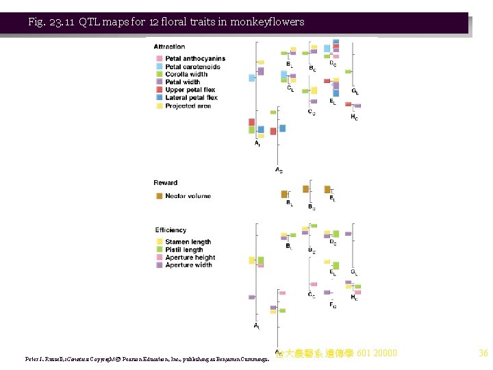
2. The number of genes involved in quantitative traits, the size of their effects and their location on the genome are being investigated using this technique. a. Identification of QTLs responsible for differences between species have emerged from this work. b. In plants, important species differences include the suites of traits that attract pollinators (color, shape, odor, nectar rewards). Monkeyflowers are an example, with pollinators ranging from hummingbirds to bees, and corresponding changes in traits (Figure 23. 11). i. Mimulus cardinalis has red color, deep nectar tubes with abundant nectar and reflexed petals. It is a hummingbird pollinated species. ii. M. lewisii has pink flowers, broad petals and little nectar reward. It is a bee pollinated species. iii. Crosses between these species show that many genes are involved, some with large effects, and many of the QTLs are physically close in the genome, indicating genetic correlation. 台大農藝系 遺傳學 601 20000 35

Fig. 23. 11 QTL maps for 12 floral traits in monkeyflowers Peter J. Russell, i. Genetics: Copyright © Pearson Education, Inc. , publishing as Benjamin Cummings. 台大農藝系 遺傳學 601 20000 36

Heritability 1. Heritability is the proportion of a population’s phenotypic variation attributable to genetic factors. 2. Continuous traits are often determined by multiple genes and by environmental factors. a. Many ecologically important traits (e. g. , body size, fecundity, development rate) are polygenic, and understanding them will contribute to knowledge of how natural populations evolve. b. Understanding the roles of genetics and environment in human health (e. g. , blood pressure, birth weight) will lead to better health care. c. Human social behaviors (e. g. , alcoholism, criminality) may also have genetic components, and scientific information has the potential to be misused in constructing social policy. 3. Heritability can be divided into two types, broad-sense and narrowsense. To assess heritability: a. Measure the variation in the trait. 台大農藝系 遺傳學 601 20000 causes. b. Partition the variance into components attributable to different 37

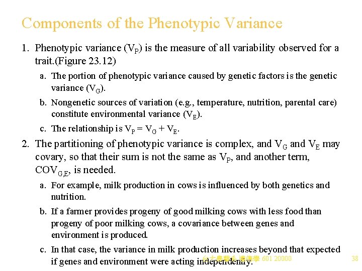
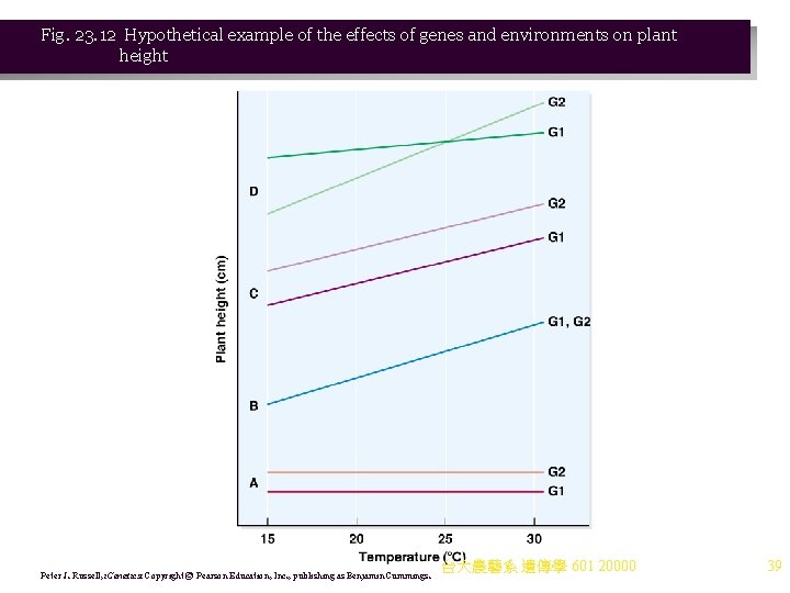
Components of the Phenotypic Variance 1. Phenotypic variance (VP) is the measure of all variability observed for a trait. (Figure 23. 12) a. The portion of phenotypic variance caused by genetic factors is the genetic variance (VG). b. Nongenetic sources of variation (e. g. , temperature, nutrition, parental care) constitute environmental variance (VE). c. The relationship is VP = VG + VE. 2. The partitioning of phenotypic variance is complex, and VG and VE may covary, so that their sum is not the same as VP, and another term, COVG, E, is needed. a. For example, milk production in cows is influenced by both genetics and nutrition. b. If a farmer provides progeny of good milking cows with less food than progeny of poor milking cows, a covariance between genes and environment is produced. c. In that case, the variance in milk production increases beyond that expected 台大農藝系 遺傳學 601 20000 if genes and environment were acting independently. 38

Fig. 23. 12 Hypothetical example of the effects of genes and environments on plant height Peter J. Russell, i. Genetics: Copyright © Pearson Education, Inc. , publishing as Benjamin Cummings. 台大農藝系 遺傳學 601 20000 39

3. Knowledge that there is a genetic component to a trait does not allow accurate predictions about offspring. Another analysis method for phenotypic variance, genotype-byenvironment (G X E) interaction, is needed. a. G X E variance exists when the relative effects of the genotypes differ among environments b. An example is temperature affecting plant height: i. In a cold environment, height of genotype AA plants averages 40 cm, while those with genotype Aa are 35 cm. ii. In a warm climate, genotype AA is 50 cm tall, while genotype Aa is now 60 cm. iii. Both genotypes grow taller in warm temperatures (an environmental effect). There is also a genetic effect, but it depends on the environment. Genetic-environmental interaction is represented by VGx E. 台大農藝系 遺傳學 601 20000 40

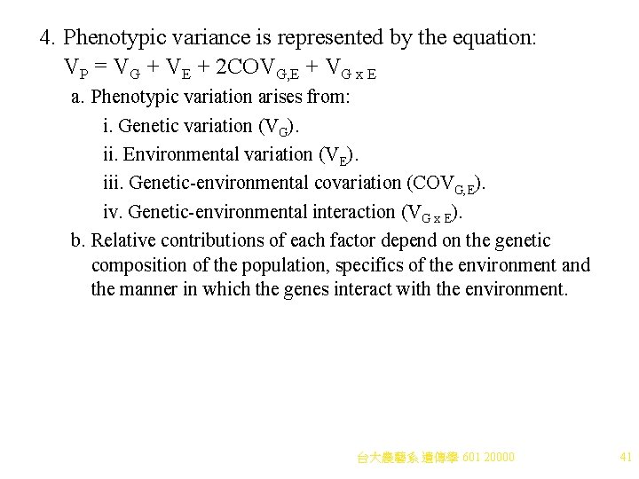
4. Phenotypic variance is represented by the equation: VP = VG + VE + 2 COVG, E + VG x E a. Phenotypic variation arises from: i. Genetic variation (VG). ii. Environmental variation (VE). iii. Genetic-environmental covariation (COVG, E). iv. Genetic-environmental interaction (VG x E). b. Relative contributions of each factor depend on the genetic composition of the population, specifics of the environment and the manner in which the genes interact with the environment. 台大農藝系 遺傳學 601 20000 41

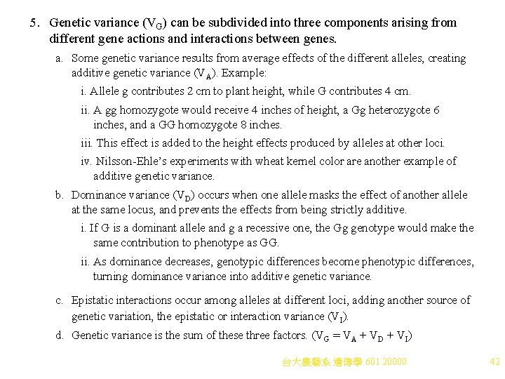
5. Genetic variance (VG) can be subdivided into three components arising from different gene actions and interactions between genes. a. Some genetic variance results from average effects of the different alleles, creating additive genetic variance (VA). Example: i. Allele g contributes 2 cm to plant height, while G contributes 4 cm. ii. A gg homozygote would receive 4 inches of height, a Gg heterozygote 6 inches, and a GG homozygote 8 inches. iii. This effect is added to the height effects produced by alleles at other loci. iv. Nilsson-Ehle’s experiments with wheat kernel color are another example of additive genetic variance. b. Dominance variance (VD) occurs when one allele masks the effect of another allele at the same locus, and prevents the effects from being strictly additive. i. If G is a dominant allele and g a recessive one, the Gg genotype would make the same contribution to phenotype as GG. ii. As dominance decreases, genotypic differences become phenotypic differences, turning dominance variance into additive genetic variance. c. Epistatic interactions occur among alleles at different loci, adding another source of genetic variation, the epistatic or interaction variance (VI). d. Genetic variance is the sum of these three factors. (VG = VA + VD + VI) 台大農藝系 遺傳學 601 20000 42

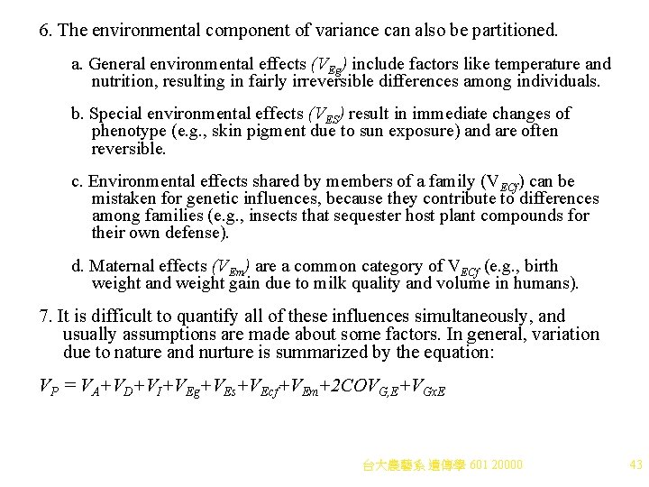
6. The environmental component of variance can also be partitioned. a. General environmental effects (VEg) include factors like temperature and nutrition, resulting in fairly irreversible differences among individuals. b. Special environmental effects (VES) result in immediate changes of phenotype (e. g. , skin pigment due to sun exposure) and are often reversible. c. Environmental effects shared by members of a family (VECf) can be mistaken for genetic influences, because they contribute to differences among families (e. g. , insects that sequester host plant compounds for their own defense). d. Maternal effects (VEm) are a common category of VECf (e. g. , birth weight and weight gain due to milk quality and volume in humans). 7. It is difficult to quantify all of these influences simultaneously, and usually assumptions are made about some factors. In general, variation due to nature and nurture is summarized by the equation: VP = VA+VD+VI+VEg+VEs+VEcf+VEm+2 COVG, E+VGx. E 台大農藝系 遺傳學 601 20000 43

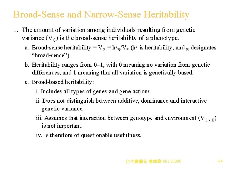
Broad-Sense and Narrow-Sense Heritability 1. The amount of variation among individuals resulting from genetic variance (VG) is the broad-sense heritability of a phenotype. a. Broad-sense heritability = VG = h 2 B/VP (h 2 is heritability, and B designates “broad-sense”). b. Heritability ranges from 0– 1, with 0 meaning no variation from genetic differences, and 1 meaning that all variation is genetically based. c. Broad-based heritability: i. Includes all types of genes and gene actions. ii. Does not distinguish between additive, dominance and interactive genetic variance. iii. Assumes that interaction between genotype and environment (VG x E) is not important. iv. Is therefore of questionable usefulness. 台大農藝系 遺傳學 601 20000 44

2. Additive genetic effects are more often used, because this component allows prediction of the average phenotype of the offspring when phenotypes of the parents are known. a. For example, in a cross for a trait involving a single locus: i. One parent might be 10 cm tall, with the genotype A 1 A 1, and the other parent 20 cm tall, with the genotype A 2 A 2. ii. If the alleles are additive, the F 1 (A 1 A 2) will be 15 cm tall, while if one allele is dominant, the F 1 will resemble one of the parents. b. In the same way, epistatic genes will not always contribute to the resemblance between parents and offspring. 3. Narrow-sense heritability is the proportion of the variance resulting from additive genetic variance. a. Narrow-sense heritability = VA = h 2 N/VP (h 2 is heritability, and N designates “narrow-sense”). b. VA determines resemblance across generations, and responds to selection in a predictable way. 台大農藝系 遺傳學 601 20000 45

Understanding Heritability 1. Heritability estimates have limitations that are often ignored, leading to misunderstanding and abuse. Important qualifications and limitations of heritability: a. Broad-sense heritability does not indicate the extent to which a trait is genetic. Rather, it measures the proportion of the phenotypic variance in a population resulting from genetic factors. i. For example, knowledge of football requires a nervous system, produced by genes, but differences in football knowledge are usually not due to genetic factors, so broad-sense heritability (VG) for football knowledge is zero. ii. If all individuals have the same genes at loci controlling a trait (e. g. , eye or ear number), VG = 0, even though genes are clearly involved in producing the trait. iii. High heritability also does not mean that environment is unimportant. It may mean instead that environmental factors influencing the trait are relatively uniform across the population. b. Heritability does not indicate what proportion of an individual’s phenotype is genetic. Heritability is a characteristic台大農藝系 of a population, an individual. 遺傳學 601 not 20000 46

c. Heritability is not fixed for a trait. It depends on the genetic makeup and environment of a population, and so a calculation for one group may not hold true in another. An example is human height. i. In a population with a uniformly high quality diet, differences in height are likely to be due to genetic factors, especially if there is high ethnic diversity. ii. In a population where quality of diet varies widely, height differences will be due less to genetic factors, and relatively more to environmental factors. d. High heritability for a trait does not imply that a population’s differences in the same trait are genetically determined. An example is diet in mice. i. Genetically diverse mice were randomly split into two groups. Both groups received the same space, water and other environmental necessities. The only difference was diet. (1) Mice in the group receiving nutritionally rich food grew large. Heritability of adult body weight was calculated at 0. 93. (2) Mice in the group receiving an impoverished diet lacking calories and essential nutrients were smaller. Heritability of adult body weight was 0. 93. (3) Both large size and small size were calculated to be highly heritable in these mice. This is a contradiction, since both groups are from the same genetic stock. 台大農藝系 遺傳學 601 20000 47

(4) Another example is the correlation between presence of books in the home and a child’s reading skill. e. Traits shared by members of the same family do not necessarily have high heritability. i. Familial traits may arise from either shared genes or shared environment. ii. Familiality is distinct from heritability. 台大農藝系 遺傳學 601 20000 48

How Heritability Is Calculated 1. Many of the methods used compare related and unrelated individuals, or compare individuals with different degrees of relatedness. When environmental conditions are identical: a. Closely related individuals have similar phenotypes when the trait is genetically determined. b. Related individuals are no more similar in phenotype than unrelated ones when the trait is environmentally determined. 2. In humans, environmental conditions are complex in structure, and extended parental care means that it is difficult to separate the effects of genetics from those of nurture and culture. Methods of calculating heritability in humans include: a. Comparison of parents and offspring. b. Comparison of full and half siblings. c. Comparison of identical and nonidentical twins. d. Response-to-selection data. 台大農藝系 遺傳學 601 20000 49

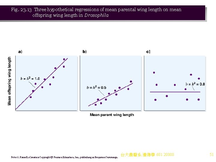
3. Heritability from parent-offspring regression is calculated by correlation and regression of data measuring the phenotypes of parents and offspring in a series of families. a. The mean phenotype of the parents (mid-parent value) and mean phenotype of offspring are plotted with each point on the graph representing one family (Figure 23. 13). i. Random scatter across the plot indicates no relationship between the traits of parents and offspring, and thus low heritability. ii. Linear relationships between phenotypes of parents and offspring indicate that heritabifity is high (unless environmental effects have influenced the trait). iii. Slope of the parent-offspring regression line reflects the magnitude of heritability. (1) If the slope is 0, narrow-sense heritability (h 2 N) is also 0. (2) If the slope is 1, offspring have a phenotype exactly intermediate between the two parents, and additive gene effects account for the entire phenotype. (3) If the slope is between 0 and 1, both additive genes and nonadditive factors (dominant and epistatic genes, environment) affect the phenotype. 台大農藝系 遺傳學 601 20000 50

Fig. 23. 13 Three hypothetical regressions of mean parental wing length on mean offspring wing length in Drosophila Peter J. Russell, i. Genetics: Copyright © Pearson Education, Inc. , publishing as Benjamin Cummings. 台大農藝系 遺傳學 601 20000 51

b. When the mean phenotype of the offspring is regressed against the phenotype of only one parent, the narrow-sense heritability is twice the slope, because the offspring shares only 1/2 its genes with the parent. c. The factor by which the slope is multiplied to obtain heritability increases as the distance between relatives increases. 4. Heritability values have been calculated for many traits in a variety of species and populations, using several methods (Table 23. 5). a. Heritability estimates are not precise and may vary widely for the same trait in the same organism. b. Human heritability values are especially difficult, because genetic and environmental factors are hard to separate. 台大農藝系 遺傳學 601 20000 52

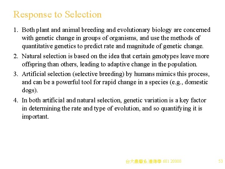
Response to Selection 1. Both plant and animal breeding and evolutionary biology are concerned with genetic change in groups of organisms, and use the methods of quantitative genetics to predict rate and magnitude of genetic change. 2. Natural selection is based on the idea that certain genotypes leave more offspring than others, leading to adaptive change in the population. 3. Artificial selection (selective breeding) by humans mimics this process, and can be a powerful tool for rapid change in a species (e. g. , domestic dogs). 4. In both artificial and natural selection, genetic variation is a key factor in determining the rate and type of evolution, and so quantifying it is important. 台大農藝系 遺傳學 601 20000 53

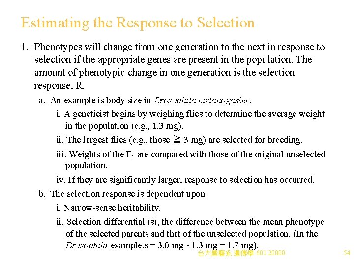
Estimating the Response to Selection 1. Phenotypes will change from one generation to the next in response to selection if the appropriate genes are present in the population. The amount of phenotypic change in one generation is the selection response, R. a. An example is body size in Drosophila melanogaster. i. A geneticist begins by weighing flies to determine the average weight in the population (e. g. , 1. 3 mg). ii. The largest flies (e. g. , those ≧ 3 mg) are selected for breeding. iii. Weights of the F 1 are compared with those of the original unselected population. iv. If they are significantly larger, response to selection has occurred. b. The selection response is dependent upon: i. Narrow-sense heritability. ii. Selection differential (s), the difference between the mean phenotype of the selected parents and that of the unselected population. (In the Drosophila example, s = 3. 0 mg - 1. 3 mg = 1. 7 mg). 台大農藝系 遺傳學 601 20000 54

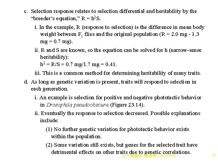
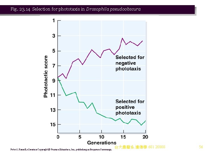
c. Selection response relates to selection differential and heritability by the “breeder’s equation, ” R = h 2 S. i. In the example, R (response to selection) is the difference in mean body weight between F 1 flies and the original population (R = 2. 0 mg - 1. 3 mg = 0. 7 mg). ii. R and S are known, so the equation can be solved for h (narrow-sense heritability): h 2 = R/S = 0. 7 mg/1. 7 mg = 0. 41. iii. This is a common method for determining heritability of many traits. d. As long as genetic variation is present, traits will respond to selection in each generation. i. An example is selection for positive and negative phototactic behavior in Drosophila pseudoobscura (Figure 23. 14). ii. Eventually the response to selection decreased. Possible explanations include: (1) No further genetic variation for phototactic behavior exists within the population. (2) Some variation still exists, but genes for the selected trait have detrimental effects on other traits due to genetic correlations. 台大農藝系 遺傳學 601 20000 55

Fig. 23. 14 Selection for phototaxis in Drosophila pseudoobscura Peter J. Russell, i. Genetics: Copyright © Pearson Education, Inc. , publishing as Benjamin Cummings. 台大農藝系 遺傳學 601 20000 56

Genetic Correlations 1. Phenotypes of more than one trait may be correlated, and therefore do not vary independently (e. g. , blond hair, fair skin and blue eyes). Association is not complete, but the traits are found together more often than chance predicts. a. Phenotypic correlation is computed by measuring the two phenotypes in a number of individuals, and then calculating a correlation coefficient for the two traits. b. Sometimes phenotypic correlation occurs because the traits are influenced by a common set of genes (e. g. , human hair, eye and skin color). c. A gene affecting ≧ 2 traits is pleiotropic, and the traits will be correlated (e. g. , human height and weight). d. Environmental factors may also cause nonrandom associations between phenotypes (e. g. , fertilizing soil may cause taller plants with more flowers). 台大農藝系 遺傳學 601 20000 57

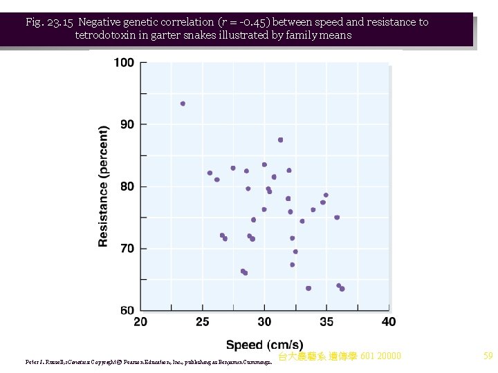
2. Genetic correlations may be positive or negative. a. Positive correlation means increase in one trait correlates with an increase in the other (e. g. , body and egg weight in chickens). b. Negative correlation means an increase in one trait correlates with a decrease in the other (e. g. , egg size and number of eggs laid). Negative correlations represent trade-offs (genetic constraints). Examples include: i. Garter snakes, where for unknown reasons speed in escaping predators correlates negatively with resistance to toxic newts in the diet. ii. Dairy cattle, where milk yield correlates negatively with butterfat content. 3. Ability to adapt to a particular environment is also often influenced by genetic correlations among traits. An example is tadpoles, where developmental rate and size at metamorphosis show a negative correlation. a. Genes that accelerate development (a good thing for life in a puddle that may dry up quickly) cause metamorphosis to occur in smaller tadpoles, producing smaller frogs. b. Smaller frogs have decreased survival due to water loss, predation and difficulty in finding food, and so there are constraints on the genes that accelerate development. 台大農藝系 601 20000 4. Additional examples of genetic correlations appear遺傳學 in Table 23. 7. 58

Fig. 23. 15 Negative genetic correlation (r = -0. 45) between speed and resistance to tetrodotoxin in garter snakes illustrated by family means Peter J. Russell, i. Genetics: Copyright © Pearson Education, Inc. , publishing as Benjamin Cummings. 台大農藝系 遺傳學 601 20000 59