Partial Face Recognition S Liao A K Jain

Partial Face Recognition S. Liao, A. K. Jain, and S. Z. Li, "Partial Face Recognition: Alignment-Free Approach", IEEE Transactions on Pattern Analysis and Machine Intelligence, Vol. 35, No. 5, pp. 1193 -1205, May 2013, doi: 10. 1109/TPAMI. 2012. 191

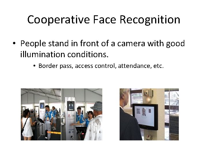
Cooperative Face Recognition • People stand in front of a camera with good illumination conditions. • Border pass, access control, attendance, etc.

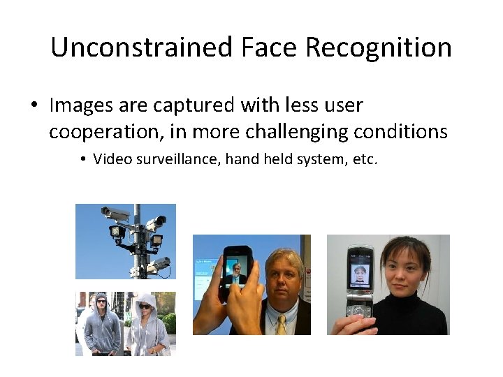
Unconstrained Face Recognition • Images are captured with less user cooperation, in more challenging conditions • Video surveillance, hand held system, etc.

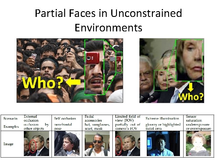
Partial Faces in Unconstrained Environments

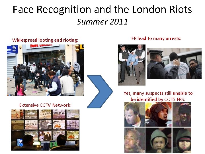
Face Recognition and the London Riots Summer 2011 Widespread looting and rioting: Extensive CCTV Network: FR lead to many arrests: Yet, many suspects still unable to be identified by COTS FRS:

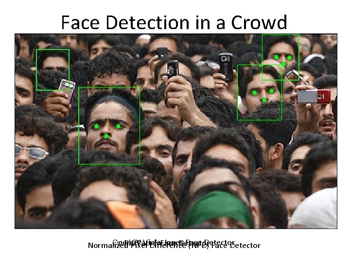
Face Detection in a Crowd Open. CV Viola-Jones Face Detector Pitt. Patt-5 Face Detector Normalized Pixel Difference (NPD) Face Detector

Unconstrained Face Recognition • Problem: – Recognize an arbitrary face image captured in unconstrained environment • Possible areas for improvement: – Face detection? – Alignment? – Feature representation? – Classification? • Importance: – Recognize a suspect in crowd – Identify a face from its partial image

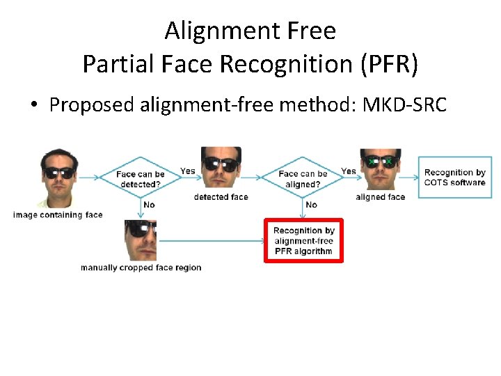
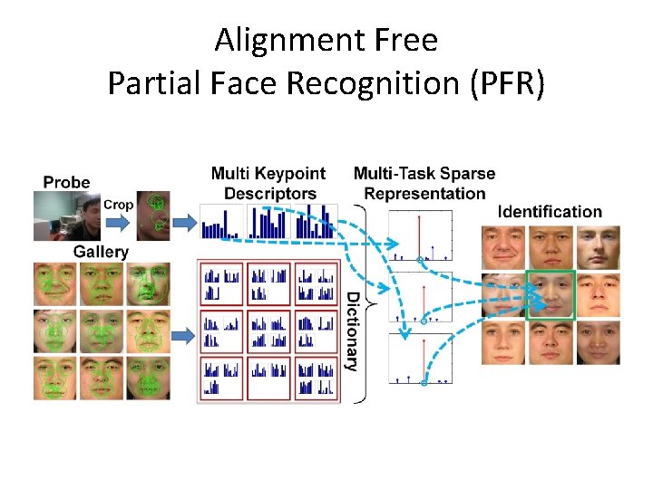
Alignment Free Partial Face Recognition (PFR) • Proposed alignment-free method: MKD-SRC

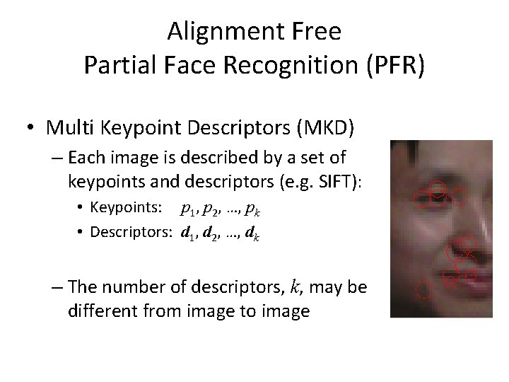
Alignment Free Partial Face Recognition (PFR) • Multi Keypoint Descriptors (MKD) – Each image is described by a set of keypoints and descriptors (e. g. SIFT): • Keypoints: p 1, p 2, …, pk • Descriptors: d 1, d 2, …, dk – The number of descriptors, k, may be different from image to image

Alignment Free Partial Face Recognition (PFR)

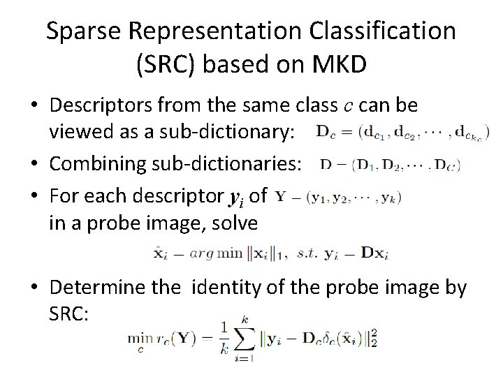
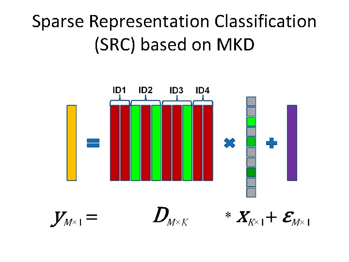
Sparse Representation Classification (SRC) based on MKD • Descriptors from the same class c can be viewed as a sub-dictionary: • Combining sub-dictionaries: • For each descriptor yi of in a probe image, solve • Determine the identity of the probe image by SRC:

Sparse Representation Classification (SRC) based on MKD

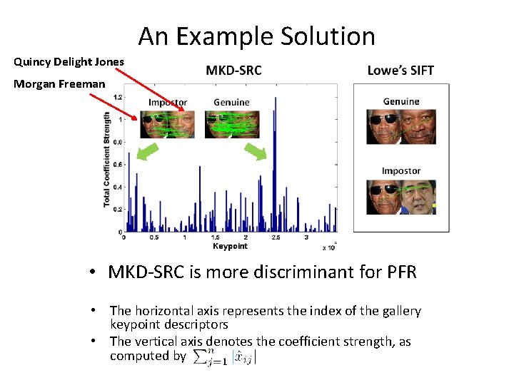
An Example Solution Quincy Delight Jones Morgan Freeman • MKD-SRC is more discriminant for PFR • The horizontal axis represents the index of the gallery keypoint descriptors • The vertical axis denotes the coefficient strength, as computed by

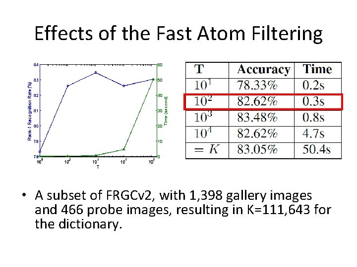
Large Scale Partial Face Recognition • In the dictionary, the number of atoms, K, can be of the order of millions • Fast atom filtering: (*) For each yi, we filter out only T (T<<K) atoms according to the top T largest values in ci, resulting in a small sub-dictionary. • The computation of Eq. (*) is linear w. r. t. K, the selection of the largest T values can be done in O(K), thus the proposed fast atom filtering scales linearly w. r. t. K, while the remaining computation of l 1 minimization takes a constant time.

Effects of the Fast Atom Filtering • A subset of FRGCv 2, with 1, 398 gallery images and 466 probe images, resulting in K=111, 643 for the dictionary.

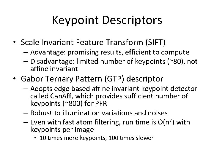
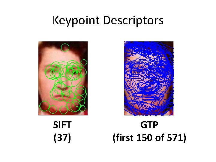
Keypoint Descriptors • Scale Invariant Feature Transform (SIFT) – Advantage: promising results, efficient to compute – Disadvantage: limited number of keypoints (~80), not affine invariant • Gabor Ternary Pattern (GTP) descriptor – Adopts edge based affine invariant keypoint detector called Can. Aff, which provides sufficient number of keypoints (~800) for PFR – Robust to illumination variations and noises – Even with fast atom filtering, run time is O(n 2) with keypoints per image • 10 times more keypoints, 100 times slower

Keypoint Descriptors SIFT (37) GTP (first 150 of 571)

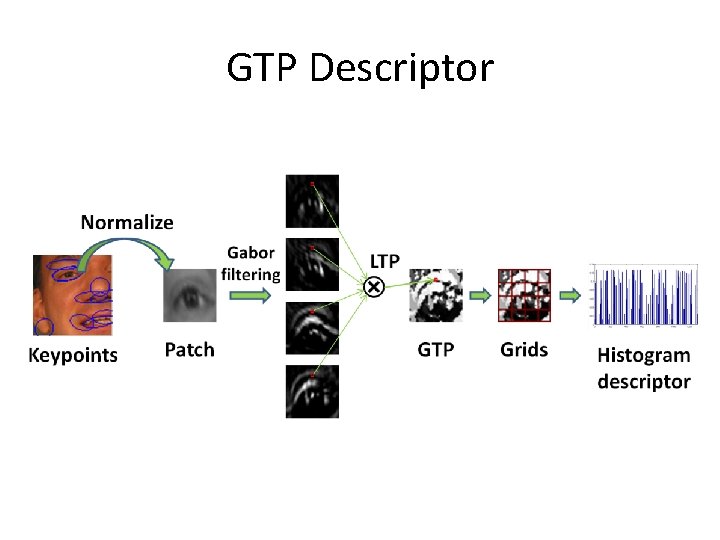
GTP Descriptor

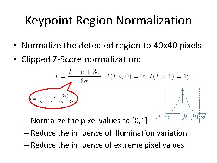
Keypoint Region Normalization • Normalize the detected region to 40 x 40 pixels • Clipped Z-Score normalization: – Normalize the pixel values to [0, 1] – Reduce the influence of illumination variation – Reduce the influence of extreme pixel values

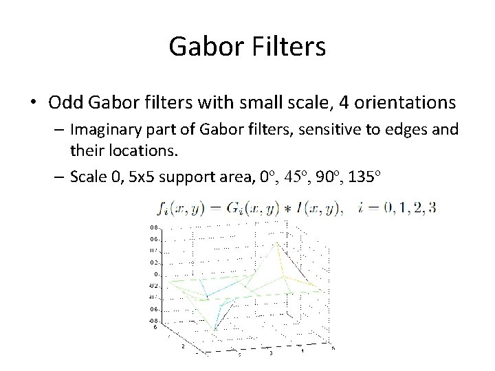
Gabor Filters • Odd Gabor filters with small scale, 4 orientations – Imaginary part of Gabor filters, sensitive to edges and their locations. – Scale 0, 5 x 5 support area, 0º, 45º, 90º, 135º

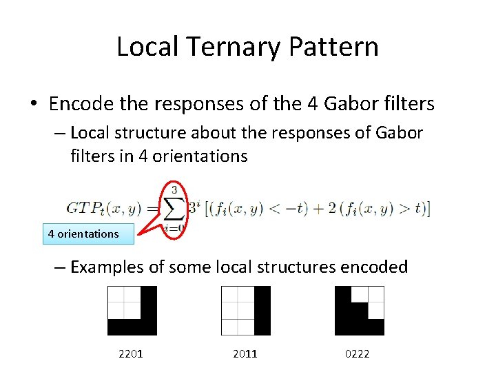
Local Ternary Pattern • Encode the responses of the 4 Gabor filters – Local structure about the responses of Gabor filters in 4 orientations – Examples of some local structures encoded 2201 2011 0222

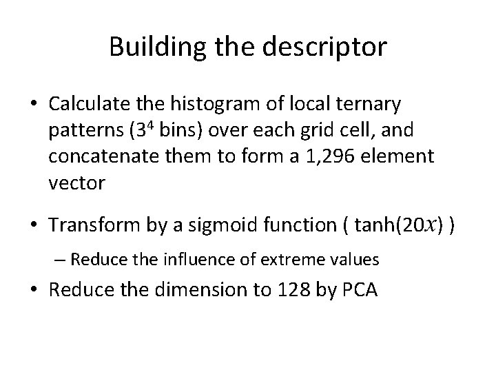
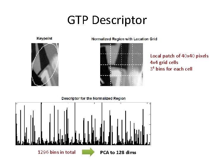
Building the descriptor • Calculate the histogram of local ternary patterns (34 bins) over each grid cell, and concatenate them to form a 1, 296 element vector • Transform by a sigmoid function ( tanh(20 x) ) – Reduce the influence of extreme values • Reduce the dimension to 128 by PCA

GTP Descriptor Local patch of 40 x 40 pixels 4 x 4 grid cells 34 bins for each cell 1296 bins in total PCA to 128 dims

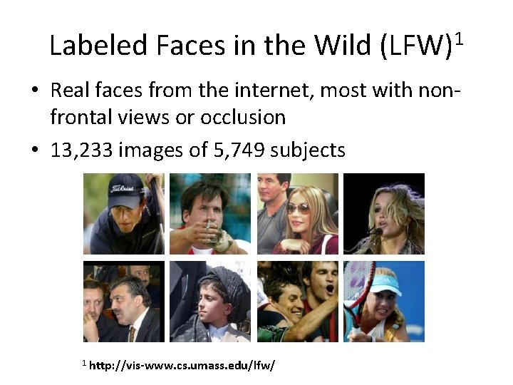
1 Labeled Faces in the Wild (LFW) • Real faces from the internet, most with nonfrontal views or occlusion • 13, 233 images of 5, 749 subjects 1 http: //vis-www. cs. umass. edu/lfw/

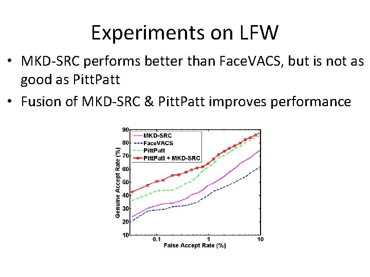
Experiments on LFW • MKD-SRC performs better than Face. VACS, but is not as good as Pitt. Patt • Fusion of MKD-SRC & Pitt. Patt improves performance

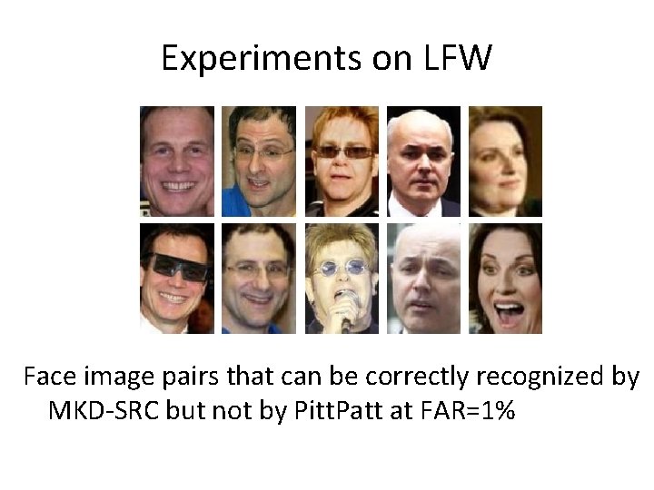
Experiments on LFW Face image pairs that can be correctly recognized by MKD-SRC but not by Pitt. Patt at FAR=1%

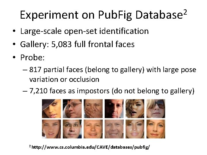
2 Experiment on Pub. Fig Database • Large-scale open-set identification • Gallery: 5, 083 full frontal faces • Probe: – 817 partial faces (belong to gallery) with large pose variation or occlusion – 7, 210 faces as impostors (do not belong to gallery) 2 http: //www. cs. columbia. edu/CAVE/databases/pubfig/

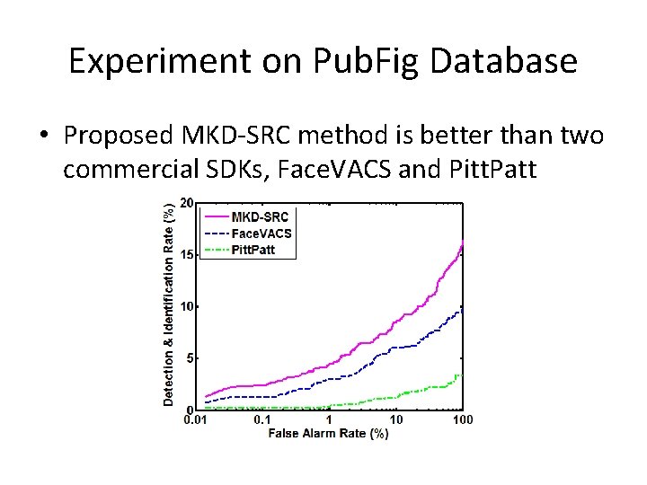
Experiment on Pub. Fig Database • Proposed MKD-SRC method is better than two commercial SDKs, Face. VACS and Pitt. Patt

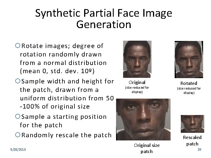
Synthetic Partial Face Image Generation Rotate images; degree of rotation randomly drawn from a normal distribution (mean 0, std. dev. 10º) Sample width and height for the patch, drawn from a uniform distribution from 50 -100% of original size Sample a starting position for the patch Randomly rescale the patch 5/28/2013 Original (size reduced for display) Original size patch Rotated (size reduced for display) Rescaled patch 29

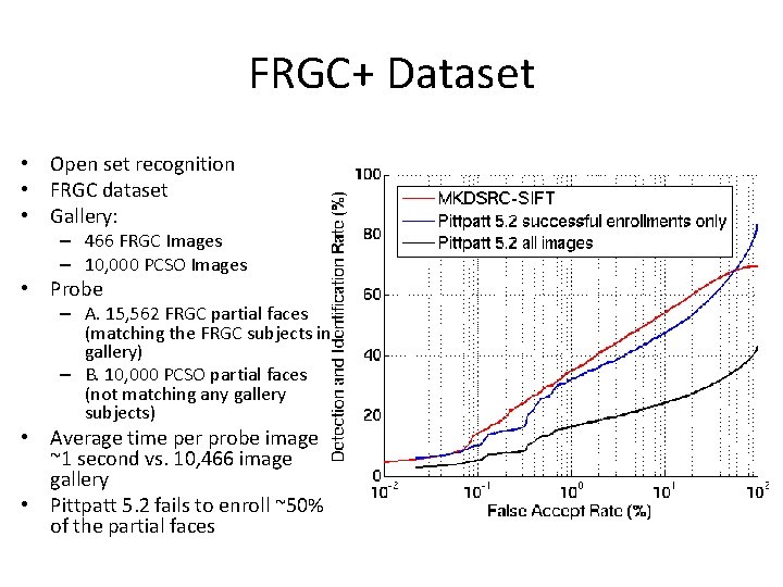
FRGC+ Dataset • Open set recognition • FRGC dataset • Gallery: – 466 FRGC Images – 10, 000 PCSO Images • Probe – A. 15, 562 FRGC partial faces (matching the FRGC subjects in gallery) – B. 10, 000 PCSO partial faces (not matching any gallery subjects) • Average time per probe image ~1 second vs. 10, 466 image gallery • Pittpatt 5. 2 fails to enroll ~50% of the partial faces

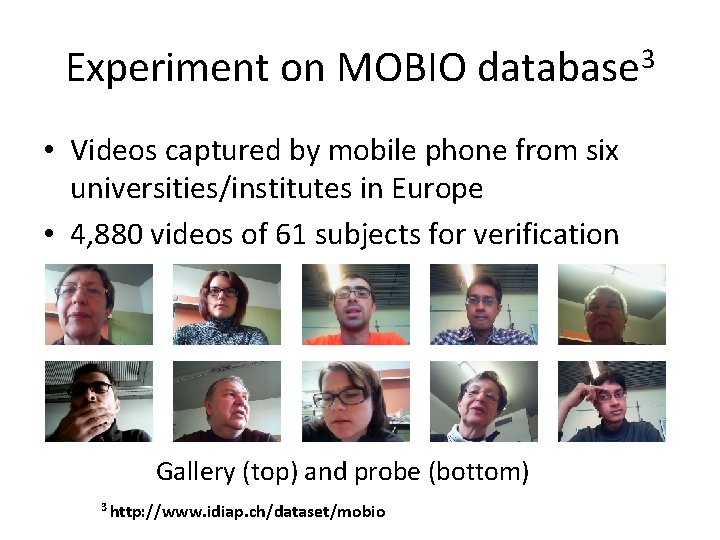
Experiment on MOBIO database 3 • Videos captured by mobile phone from six universities/institutes in Europe • 4, 880 videos of 61 subjects for verification Gallery (top) and probe (bottom) 3 http: //www. idiap. ch/dataset/mobio

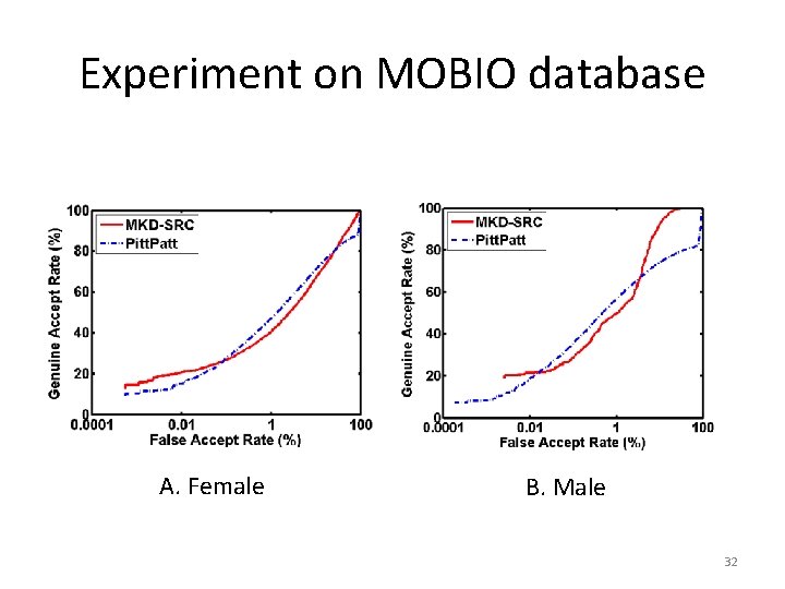
Experiment on MOBIO database A. Female B. Male 32

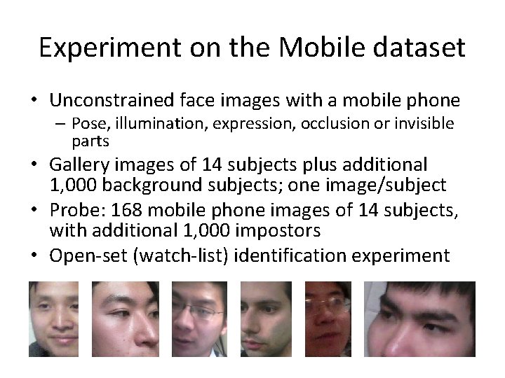
Experiment on the Mobile dataset • Unconstrained face images with a mobile phone – Pose, illumination, expression, occlusion or invisible parts • Gallery images of 14 subjects plus additional 1, 000 background subjects; one image/subject • Probe: 168 mobile phone images of 14 subjects, with additional 1, 000 impostors • Open-set (watch-list) identification experiment

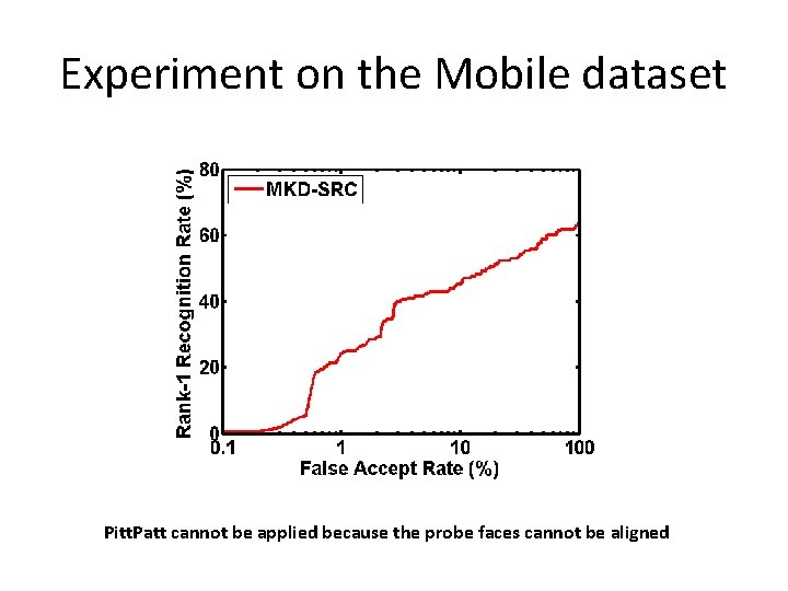
Experiment on the Mobile dataset Pitt. Patt cannot be applied because the probe faces cannot be aligned

Other Keypoint Matching Methods • Keypoint based representations are naturally variable size • The previously discussed method reconstructs each probe keypoint from the gallery using SRC • Other options: – Bag of words methods – fixed sized representation over a dictionary – Modified Hausdorff Distance – apply a general distance metric to sets of points

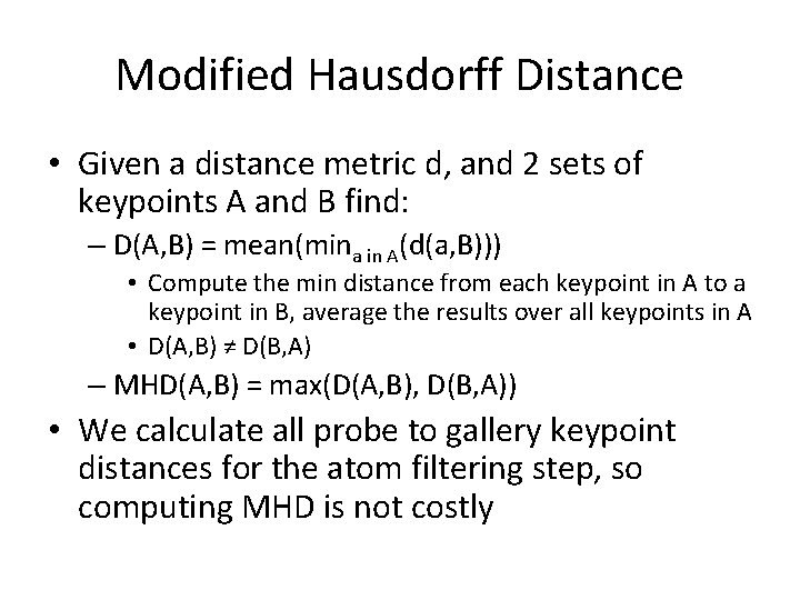
Modified Hausdorff Distance • Given a distance metric d, and 2 sets of keypoints A and B find: – D(A, B) = mean(mina in A(d(a, B))) • Compute the min distance from each keypoint in A to a keypoint in B, average the results over all keypoints in A • D(A, B) ≠ D(B, A) – MHD(A, B) = max(D(A, B), D(B, A)) • We calculate all probe to gallery keypoint distances for the atom filtering step, so computing MHD is not costly

Summary • Face recognition based on applying SRC to local keypoint descriptors • Outperformed by other methods for mugshot style images, but can be used even when faces cannot be aligned – E. g. only part of the face is available, or face/eye detection fail