FACE RECOGNITION NEHA BAIRATHI RAHUL DAGA JIGNESH DARJI

FACE RECOGNITION NEHA BAIRATHI RAHUL DAGA JIGNESH DARJI REKHA PANDA PROJECT GUIDE : - K. T. TALELE DEPARTMENT OF ELECTRONICS AND TELECOMMUNICATION BHARTIYA VIDYA BHAVAN'S SARDAR PATEL INSTITUTE OF TECHNOLOGY MUNSHI NAGAR, ANDHERI (W), MUMBAI - 400 058. 2011 -12

Roadmap • Introduction • Literature Survey Problem Definition Product Conclusion • • • 2

Introduction (1/3) �Face Recognition is a biometric approach that focuses on the same identifier that humans use primarily to distinguish one person from another: their faces. 3

Introduction (2/3) �Hollistic Method: ◦ The whole face image is used as the raw input to the recognition system. ◦ Faces are identified using global representations i. e. descriptions are based on the entire image. ◦ An example is well-known PCA which projects faces into a dimensional reduced space where recognition is carried out. 4

Introduction (3/3) �Local Feature-based Method: ◦ Local features are extracted, such as eyes, nose and mouth. ◦ The geometric relationship among the local features is computed, thus reducing the input facial image to a vector of geometric features. ◦ The locations and local statistics (appearance) are the input to the recognition stage. 5

Roadmap Introduction • Literature Survey • • Problem Definition Product Conclusion 6

Literature Survey �Local Binary Pattern(LBP) �Local Phase Quantization(LPQ) �Principal Component Analysis(PCA) �Gabor EBGM and Hog EBGM �Literature Summary 7

LBP (1/5) �Timo Ahonen and Matti Pietikainen, “Face descriptor with local binary patterns: Application to face recognition", 2006. ◦ ◦ Face is divided into sub-regions LBP is blur variant Histogram is plotted for each sub-region Each histogram is then spatially concatenated 8

LPQ (2/5) �Abdenour Hadid and Masashi Nishiyana, “Recognition of blurred faces via facial deblurring combined with blur tolerant descriptors", 2010. ◦ ◦ Face is divided into sub-regions LPQ is blur invariant Histogram is plotted for each sub-region Each histogram is then spatially concatenated 9

PCA (3/5) �Shefali Gupta, O. P. Sahu, Rupesh Gupta, Ajay Goel, “A Bespoke Approach for Face Recognition using PCA", 2010. ◦ Transform training image vector into Eigen space ◦ Euclidean distance is calculated comparing test images with training data ◦ Face is recognized if the Euclidean distance is less than threshold 10

Gabor-EBGM and Hog-EBGM (4/5) �David Monzo, Alberto Albiol, Jorge Sastre, Antonio Albiol, “Hog-EBGM vs. GABOREBGM", IEEE International Conference on Image Processing, 2010. ◦ EBGM involves localizing fiducial facial points ◦ In Gabor-EBGM, Gabor wavelet response is calculated for each point ◦ Hog-EBGM calculates Hog decriptors, which is a histogram with 128 component 11

Literature Summary (5/5) �LBP is highly sensitive to Illumination �LVQ is rotation variant �PCA is very fast but efficiency is very low �EBGM landmarks have to be calculated manually 12

Roadmap • Introduction • Literature Survey • Problem Definition • Product Conclusion • 13

Problem Definition �To design and implement a system which is less sensitive to Illumination, is rotation invariant, scale invariant and robust enough to be implemented in practical applications. 14

Roadmap • Introduction • • Literature Survey Problem Definition • Product • Conclusion 15

Product �Features �Proposed System ◦ System requirements ◦ Assumption and constraints ◦ Flow of the System �Experimental Results �Experimental Analysis 16

Features �Robust face detection �High performance matching even for large databases �Invariant to rotation, scale and illumination 17

Product �Features �Proposed System ◦ System requirements ◦ Assumption and constraints ◦ Flow of the System �Experimental Results �Experimental Analysis 18

System Requirements �USB Camera �Computer 19

Assumptions and Constraints Assumptions Constraints � Sufficient Light � Only frontal face � No sunglasses or can be detected � Twins cannot be distinguished � Tilt of the face should be less than 45 o Spectacles 20

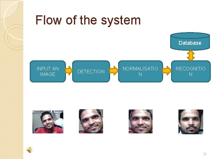
Flow of the system Database INPUT AN IMAGE DETECTION NORMALISATIO N RECOGNITIO N 21

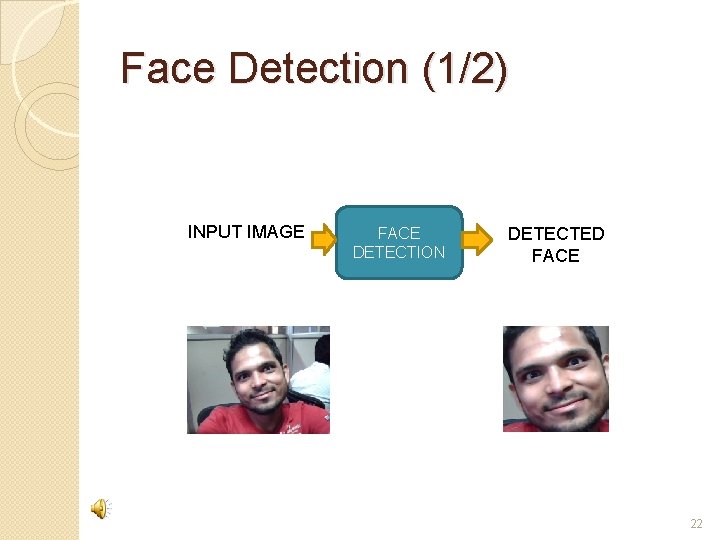
Face Detection (1/2) INPUT IMAGE FACE DETECTION DETECTED FACE 22

Face Detection (2/2) �It is implemented using ‘Object Detection Technique based on Boosted Cascade of Simple Haar-Like features’ Developed by Paul Viola and Michael Jones 23

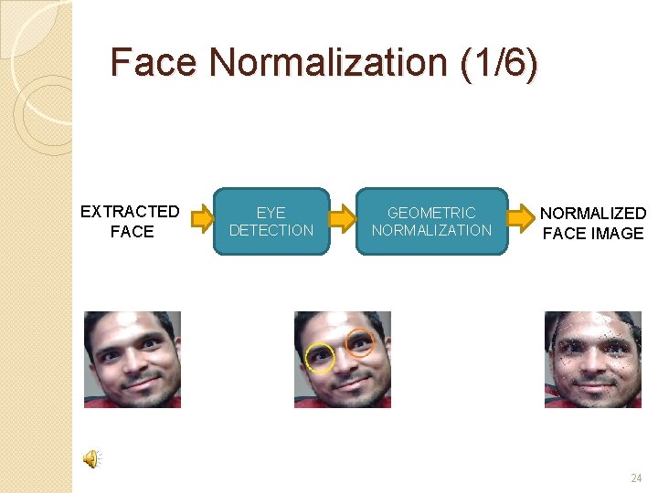
Face Normalization (1/6) EXTRACTED FACE EYE DETECTION GEOMETRIC NORMALIZATION NORMALIZED FACE IMAGE 24

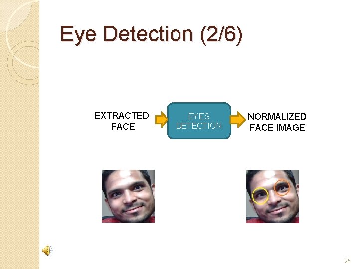
Eye Detection (2/6) EXTRACTED FACE EYES DETECTION NORMALIZED FACE IMAGE 25

Eye Detection (3/6) �It is implemented using ‘Object Detection Technique based on Boosted Cascade of Simple Haar-Like features’ Developed by Paul Viola and Michael Jones 26

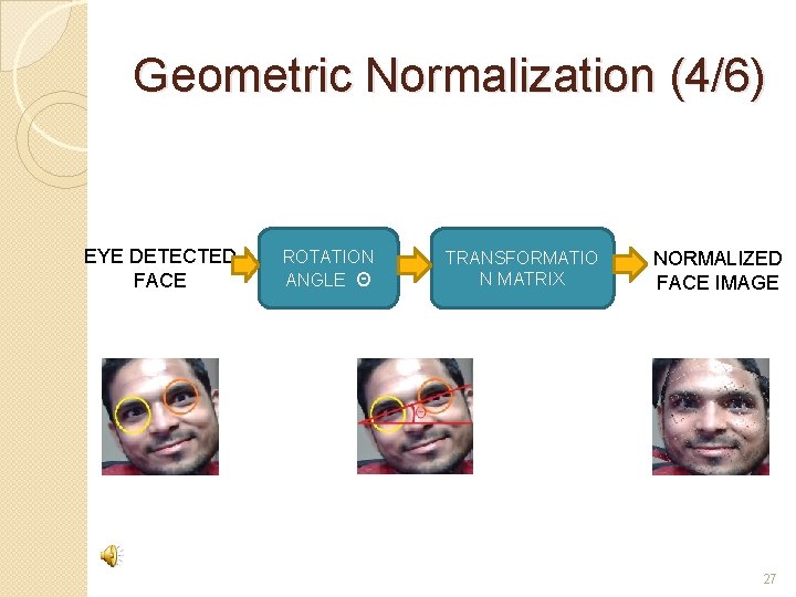
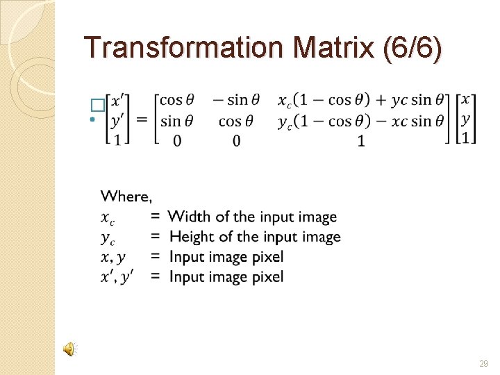
Geometric Normalization (4/6) EYE DETECTED FACE ROTATION ANGLE Θ TRANSFORMATIO N MATRIX NORMALIZED FACE IMAGE 27

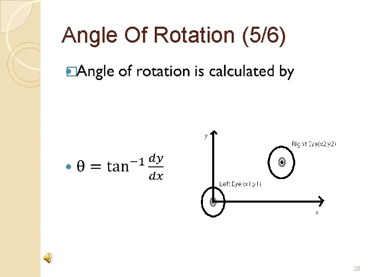
Angle Of Rotation (5/6) � 28

Transformation Matrix (6/6) � 29

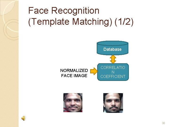
Face Recognition (Template Matching) (1/2) Database NORMALIZED FACE IMAGE CORRELATIO N COEFFICIENT 30

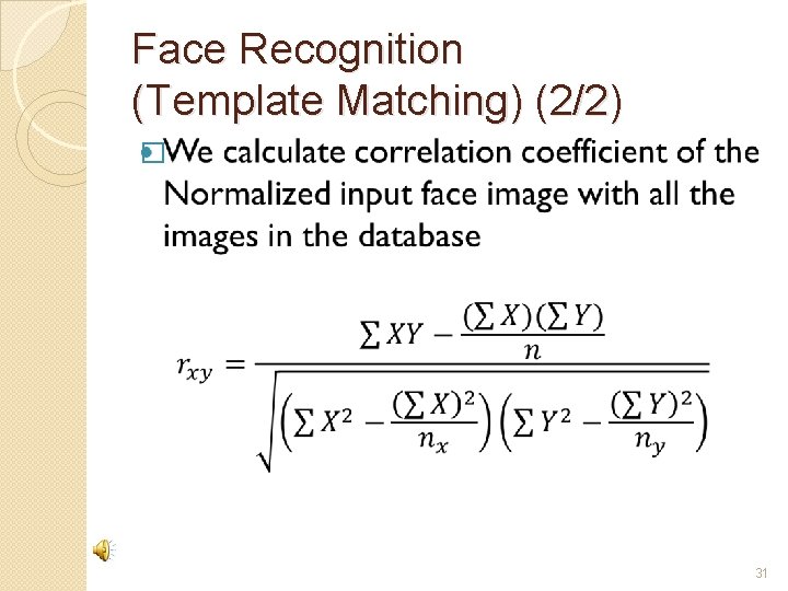
Face Recognition (Template Matching) (2/2) � 31

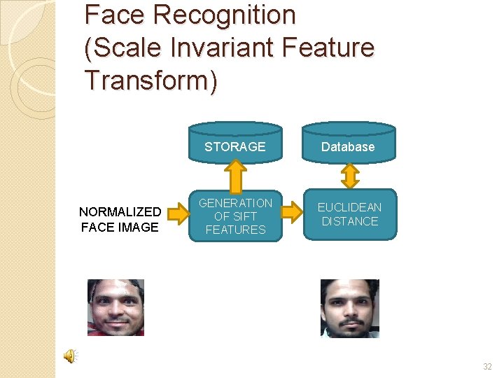
Face Recognition (Scale Invariant Feature Transform) NORMALIZED FACE IMAGE STORAGE Database GENERATION OF SIFT FEATURES EUCLIDEAN DISTANCE 32

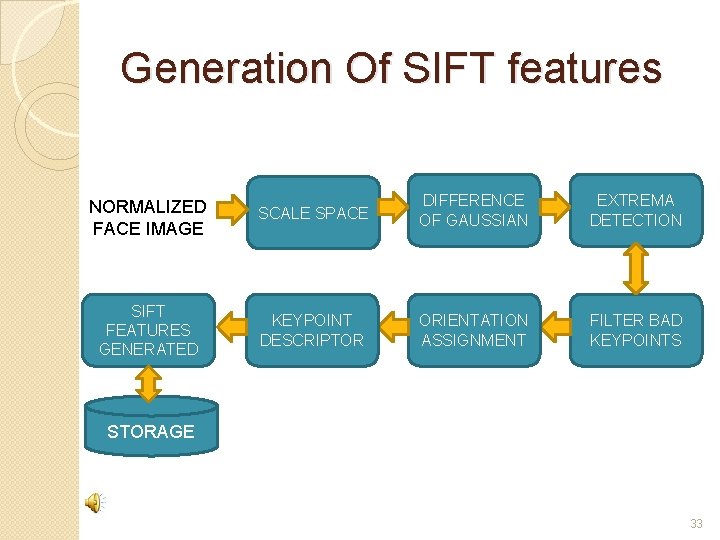
Generation Of SIFT features NORMALIZED FACE IMAGE SCALE SPACE DIFFERENCE OF GAUSSIAN EXTREMA DETECTION SIFT FEATURES GENERATED KEYPOINT DESCRIPTOR ORIENTATION ASSIGNMENT FILTER BAD KEYPOINTS STORAGE 33

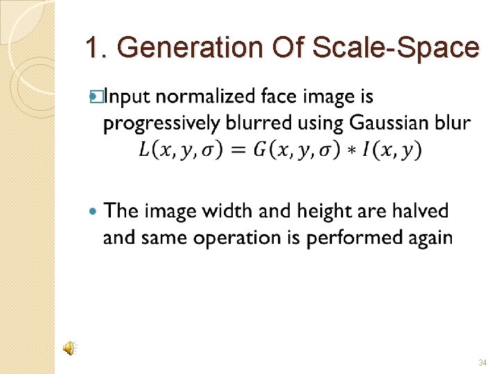
1. Generation Of Scale-Space � 34

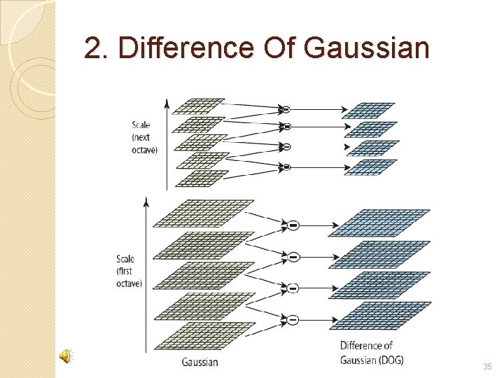
2. Difference Of Gaussian 35

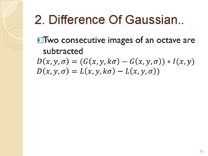
2. Difference Of Gaussian. . � 36

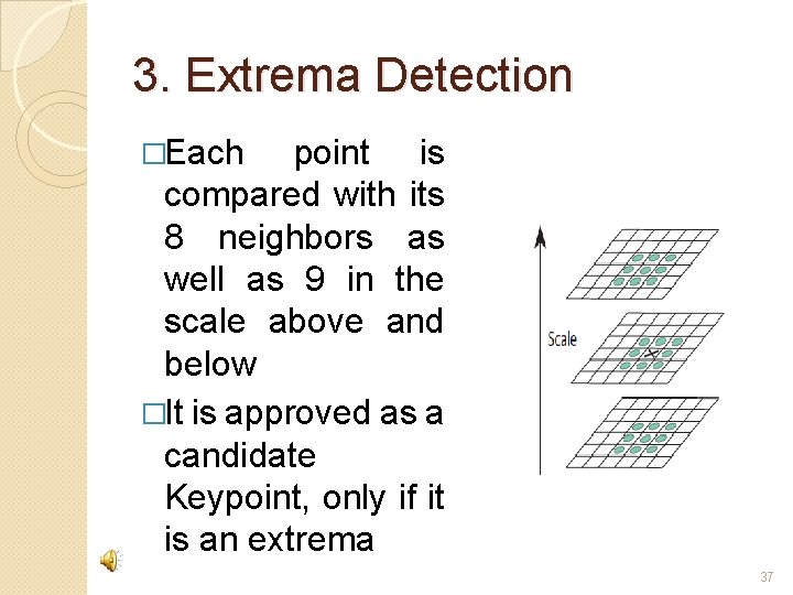
3. Extrema Detection �Each point is compared with its 8 neighbors as well as 9 in the scale above and below �It is approved as a candidate Keypoint, only if it is an extrema 37

4. Removal Of Bad Keypoints �Removal of low contrast keypoints �Removal of unstable edge keypoints 38

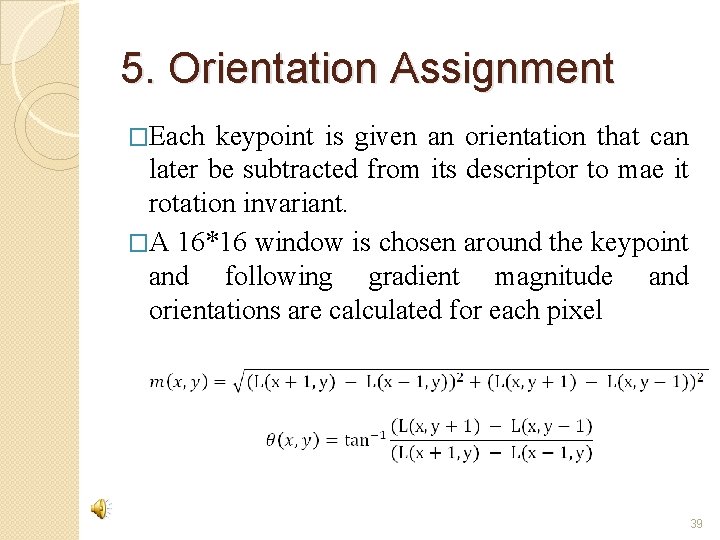
5. Orientation Assignment �Each keypoint is given an orientation that can later be subtracted from its descriptor to mae it rotation invariant. �A 16*16 window is chosen around the keypoint and following gradient magnitude and orientations are calculated for each pixel 39

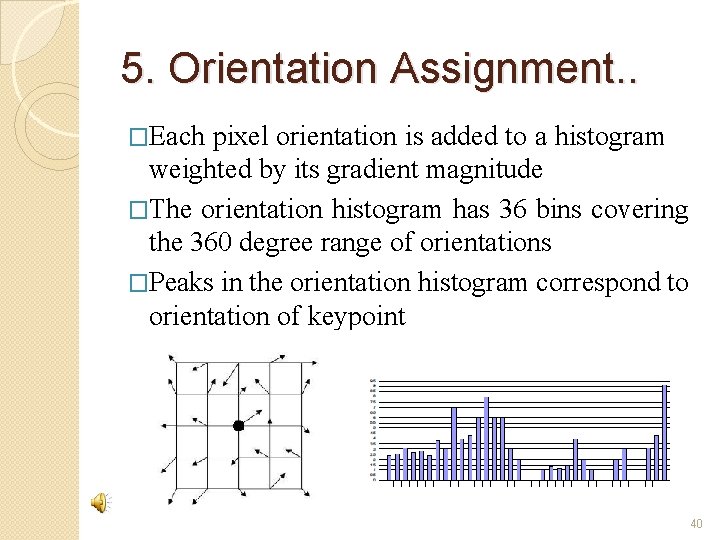
5. Orientation Assignment. . �Each pixel orientation is added to a histogram weighted by its gradient magnitude �The orientation histogram has 36 bins covering the 360 degree range of orientations �Peaks in the orientation histogram correspond to orientation of keypoint 40

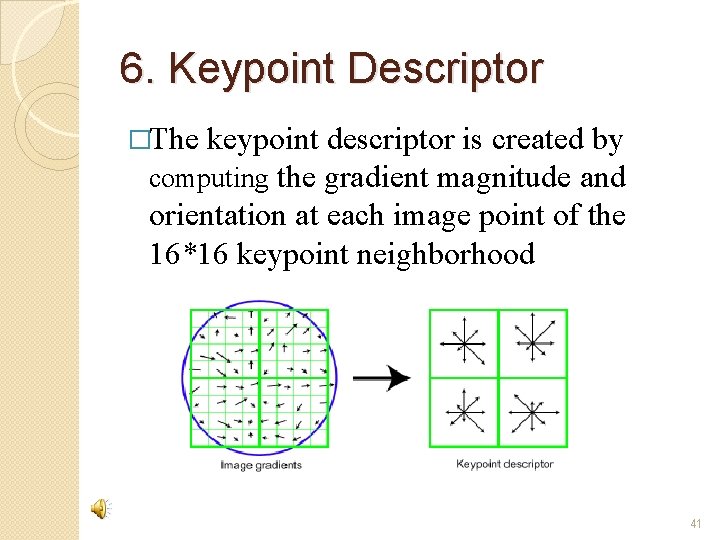
6. Keypoint Descriptor �The keypoint descriptor is created by computing the gradient magnitude and orientation at each image point of the 16*16 keypoint neighborhood 41

6. Keypoint Descriptor. . �The neighborhood is weighted by a Gaussian window and then accumulated into orientation histograms for each region of size 4*4 �Each histogram contains 8 bins, therefore each keypoint descriptor features 4 * 8 = 128 elements �The coordinates of the descriptor and the gradient orientations are rotated relative to the keypoint orientation to achieve orientation invariance 42

Euclidean Distance �Each image contains N key points and each key point has 128 descriptors �We match two key points by calculating Euclidean distance �The image from the database which has the lowest Euclidean distance with the input is the matched image 43

Product �Features �Existing System �Proposed System ◦ System requirements ◦ Assumption and constraints ◦ Flow of the System �Experimental Results �Experimental Analysis 44

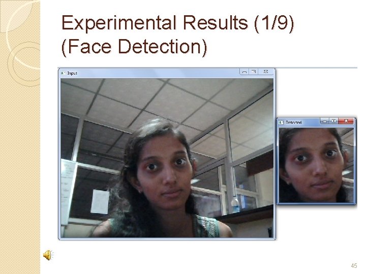
Experimental Results (1/9) (Face Detection) 45

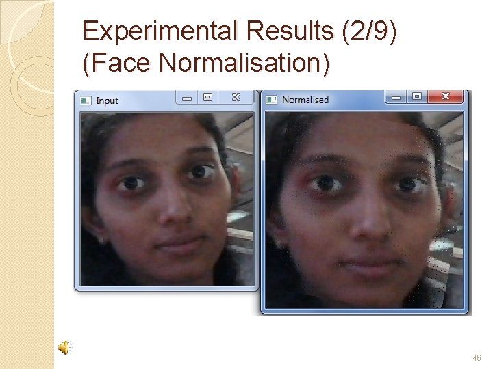
Experimental Results (2/9) (Face Normalisation) 46

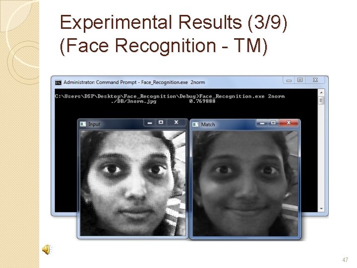
Experimental Results (3/9) (Face Recognition - TM) 47

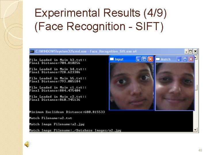
Experimental Results (4/9) (Face Recognition - SIFT) 48

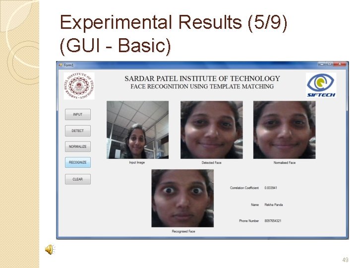
Experimental Results (5/9) (GUI - Basic) 49

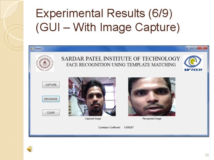
Experimental Results (6/9) (GUI – With Image Capture) 50

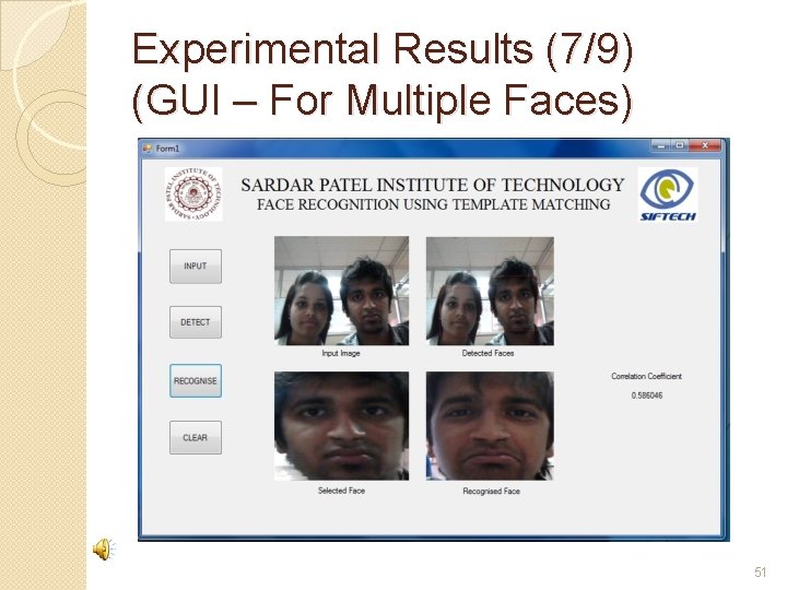
Experimental Results (7/9) (GUI – For Multiple Faces) 51

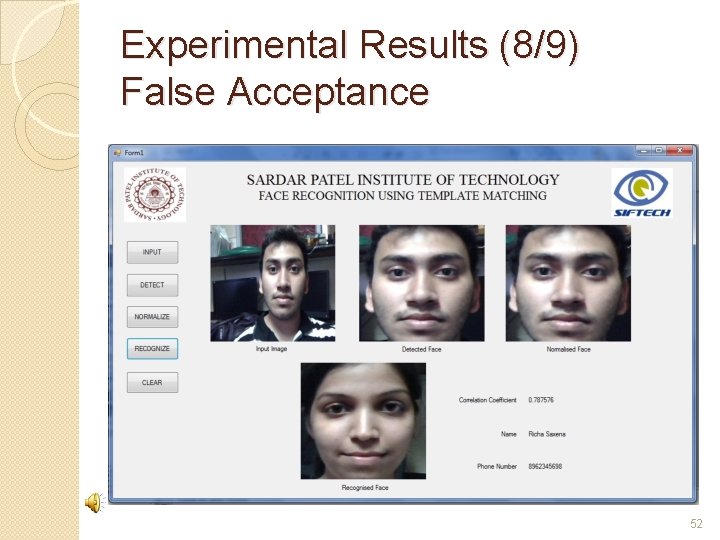
Experimental Results (8/9) False Acceptance 52

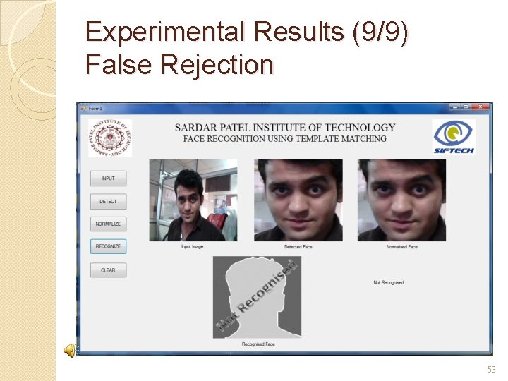
Experimental Results (9/9) False Rejection 53

Product �Features �Existing System �Proposed System ◦ System requirements ◦ Assumption and constraints ◦ Flow of the System �Experimental Results �Experimental Analysis 54

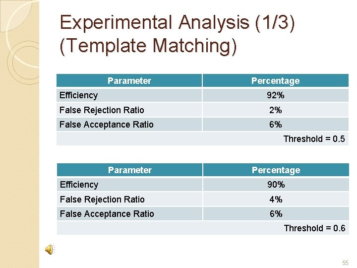
Experimental Analysis (1/3) (Template Matching) Parameter Percentage Efficiency 92% False Rejection Ratio 2% False Acceptance Ratio 6% Threshold = 0. 5 Parameter Percentage Efficiency 90% False Rejection Ratio 4% False Acceptance Ratio 6% Threshold = 0. 6 55

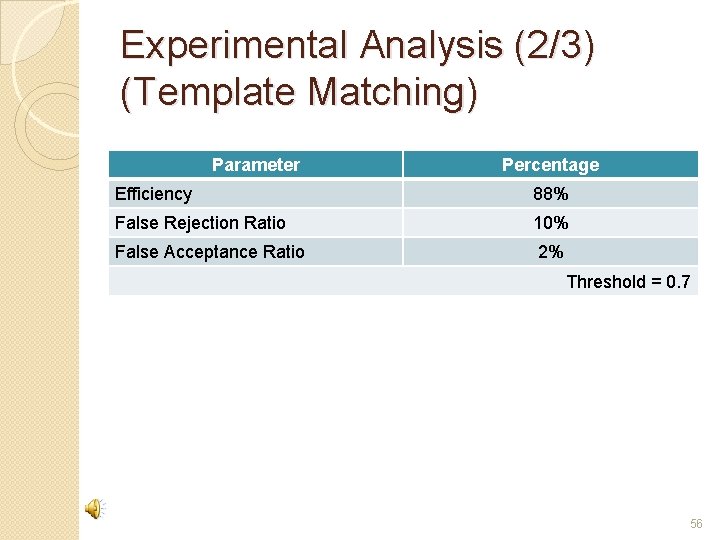
Experimental Analysis (2/3) (Template Matching) Parameter Percentage Efficiency 88% False Rejection Ratio 10% False Acceptance Ratio 2% Threshold = 0. 7 56

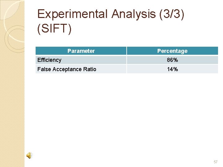
Experimental Analysis (3/3) (SIFT) Parameter Percentage Efficiency 86% False Acceptance Ratio 14% 57

Roadmap • Introduction • • Literature Survey Problem Definition Product • Conclusion • 58

Conclusion �Here we presented Face Recognition using Template Matching and Scale Invariant Feature Transform. �In Template Matching, we calculate the correlation co-efficient between two images and the image with maximum correlation coefficient is considered as the match. �In Scale Invariant Feature Transform, the keypoints are generated and are compared with the keypoints of images in the database. The comparison that gives minimum Euclidean distance is the match of the input image. 59

References � Abdenour Hadid and Masashi Nishiyana, “Recognition of blurred faces via deblurring combined with blur tolerant descriptors”, 2010. � Timo Ahonen and Matti Pietikainen, “Face descriptor with local binary patterns”, 2008. � Shefali Gupta, O. P. Sahu, Rupesh Gupta, Ajay Goel , “A Bespoke approach for Face Recognition using PCA ”, 2010. � Janez Krizag, Victomir Struc, Nikola Pavesic, “Adaption of SIFT features for robust face recognition”. 2010 � David Monzo, Alberto Albiol, Jorge Siastro, Antonio Albiol, “HOG EBGM vs. GABOR-EBGM” , 2010. � Yu meng , dr. Bernard Tiddeman, “Implementing the SIFT method” 60