CS 790 Q Biometrics Face Recognition Using Dimensionality

CS 790 Q Biometrics Face Recognition Using Dimensionality Reduction PCA and LDA M. Turk, A. Pentland, "Eigenfaces for Recognition", Journal of Cognitive Neuroscience, 3(1), pp. 71 -86, 1991. D. Swets, J. Weng, "Using Discriminant Eigenfeatures for Image Retrieval", IEEE Transactions on Pattern Analysis and Machine Intelligence, 18(8), pp. 831 -836, 1996. A. Martinez, A. Kak, "PCA versus LDA", IEEE Transactions on Pattern Analysis and Machine Intelligence, vol. 23, no. 2, pp. 228 -233, 2001.

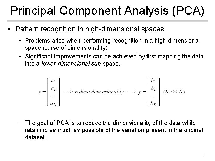
Principal Component Analysis (PCA) • Pattern recognition in high-dimensional spaces − Problems arise when performing recognition in a high-dimensional space (curse of dimensionality). − Significant improvements can be achieved by first mapping the data into a lower-dimensional sub-space. − The goal of PCA is to reduce the dimensionality of the data while retaining as much as possible of the variation present in the original dataset. 2

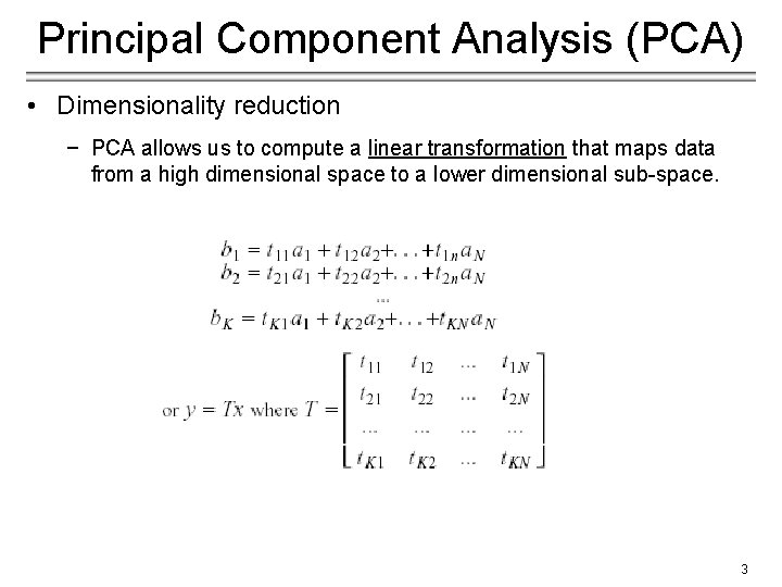
Principal Component Analysis (PCA) • Dimensionality reduction − PCA allows us to compute a linear transformation that maps data from a high dimensional space to a lower dimensional sub-space. 3

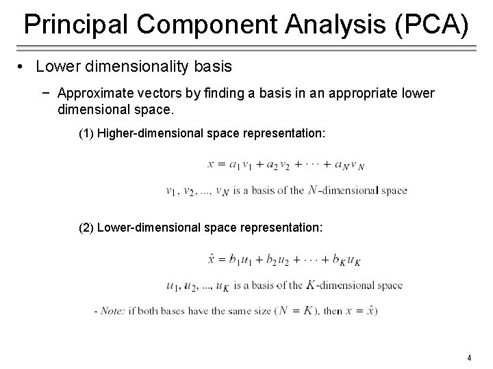
Principal Component Analysis (PCA) • Lower dimensionality basis − Approximate vectors by finding a basis in an appropriate lower dimensional space. (1) Higher-dimensional space representation: (2) Lower-dimensional space representation: 4

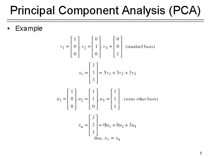
Principal Component Analysis (PCA) • Example 5

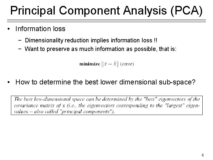
Principal Component Analysis (PCA) • Information loss − Dimensionality reduction implies information loss !! − Want to preserve as much information as possible, that is: • How to determine the best lower dimensional sub-space? 6

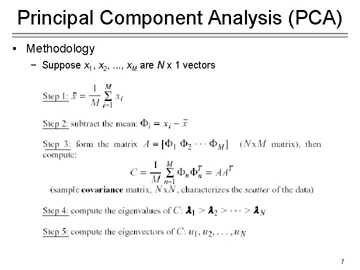
Principal Component Analysis (PCA) • Methodology − Suppose x 1, x 2, . . . , x. M are N x 1 vectors 7

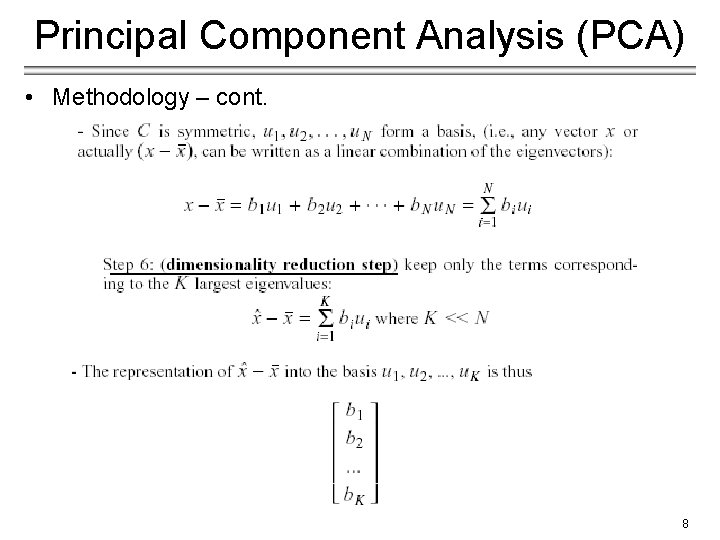
Principal Component Analysis (PCA) • Methodology – cont. 8

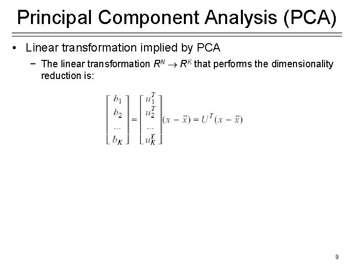
Principal Component Analysis (PCA) • Linear transformation implied by PCA − The linear transformation RN RK that performs the dimensionality reduction is: 9

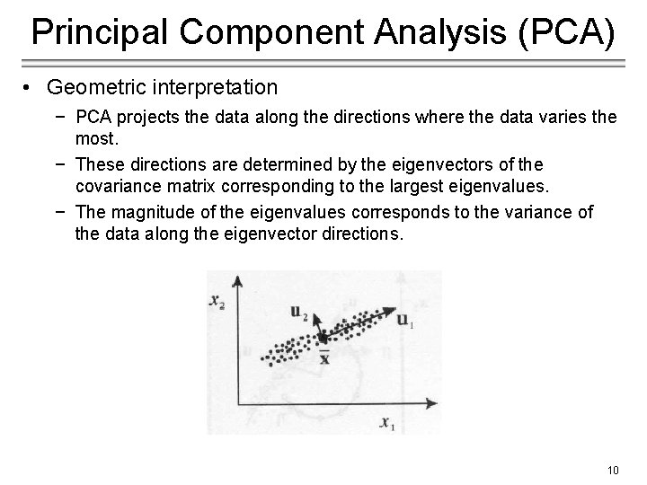
Principal Component Analysis (PCA) • Geometric interpretation − PCA projects the data along the directions where the data varies the most. − These directions are determined by the eigenvectors of the covariance matrix corresponding to the largest eigenvalues. − The magnitude of the eigenvalues corresponds to the variance of the data along the eigenvector directions. 10

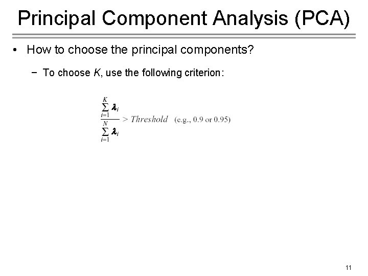
Principal Component Analysis (PCA) • How to choose the principal components? − To choose K, use the following criterion: 11

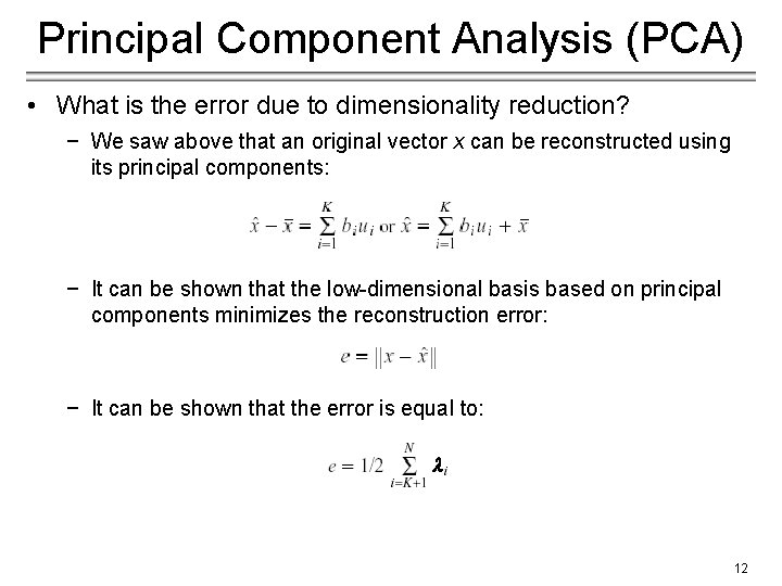
Principal Component Analysis (PCA) • What is the error due to dimensionality reduction? − We saw above that an original vector x can be reconstructed using its principal components: − It can be shown that the low-dimensional basis based on principal components minimizes the reconstruction error: − It can be shown that the error is equal to: 12

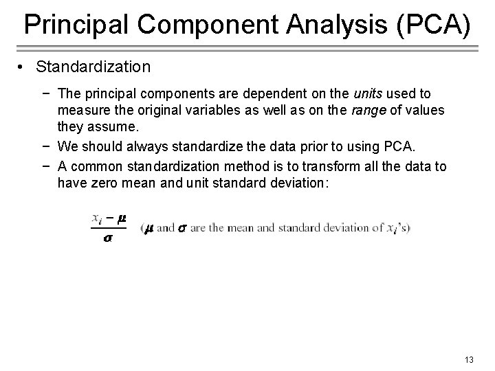
Principal Component Analysis (PCA) • Standardization − The principal components are dependent on the units used to measure the original variables as well as on the range of values they assume. − We should always standardize the data prior to using PCA. − A common standardization method is to transform all the data to have zero mean and unit standard deviation: 13

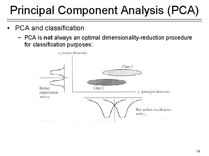
Principal Component Analysis (PCA) • PCA and classification − PCA is not always an optimal dimensionality-reduction procedure for classification purposes: 14

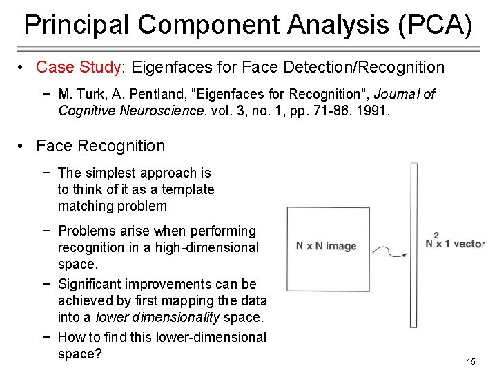
Principal Component Analysis (PCA) • Case Study: Eigenfaces for Face Detection/Recognition − M. Turk, A. Pentland, "Eigenfaces for Recognition", Journal of Cognitive Neuroscience, vol. 3, no. 1, pp. 71 -86, 1991. • Face Recognition − The simplest approach is to think of it as a template matching problem − Problems arise when performing recognition in a high-dimensional space. − Significant improvements can be achieved by first mapping the data into a lower dimensionality space. − How to find this lower-dimensional space? 15

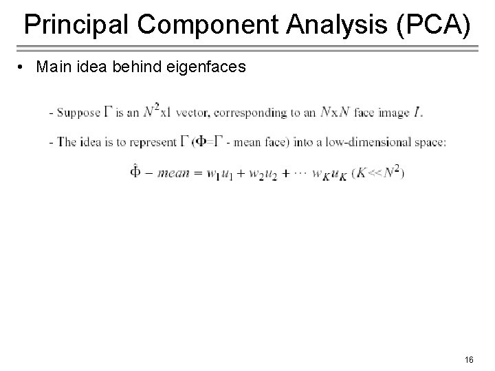
Principal Component Analysis (PCA) • Main idea behind eigenfaces 16

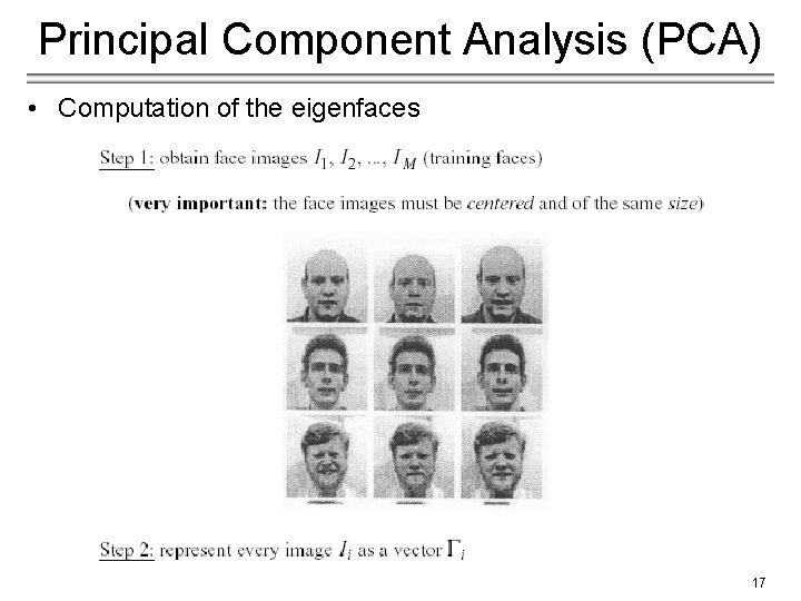
Principal Component Analysis (PCA) • Computation of the eigenfaces 17

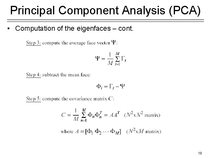
Principal Component Analysis (PCA) • Computation of the eigenfaces – cont. 18

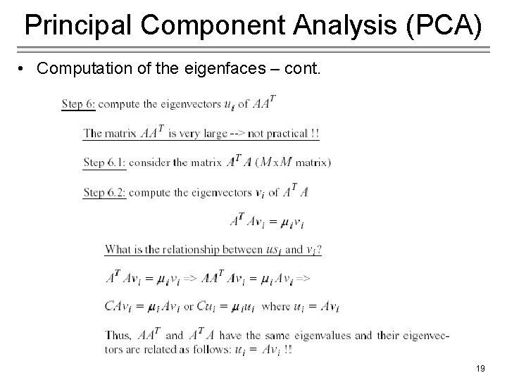
Principal Component Analysis (PCA) • Computation of the eigenfaces – cont. 19

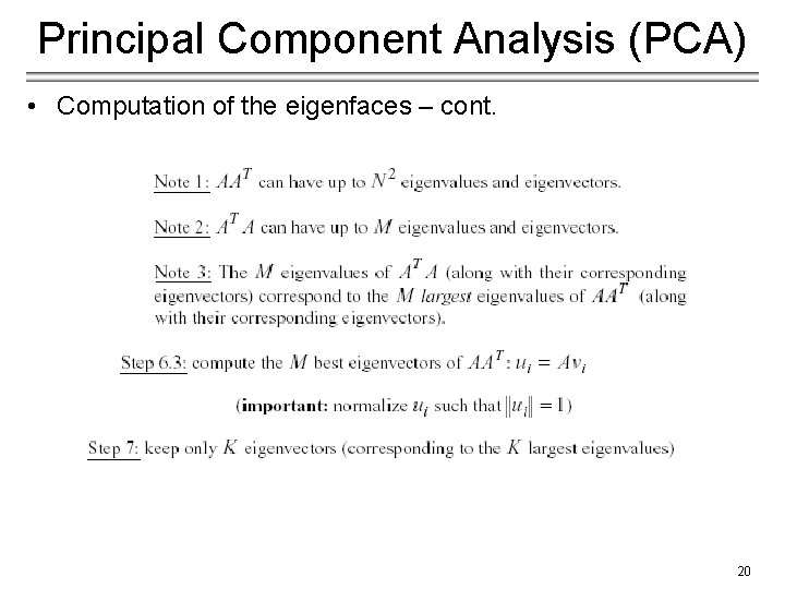
Principal Component Analysis (PCA) • Computation of the eigenfaces – cont. 20

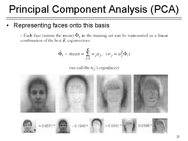
Principal Component Analysis (PCA) • Representing faces onto this basis 21

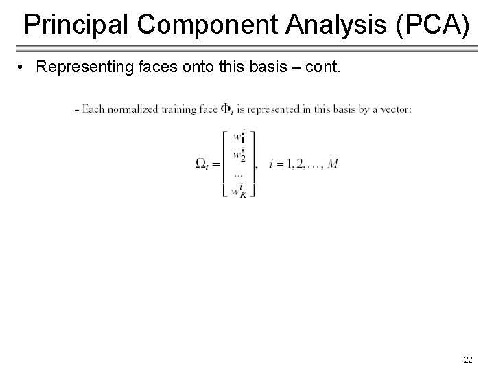
Principal Component Analysis (PCA) • Representing faces onto this basis – cont. 22

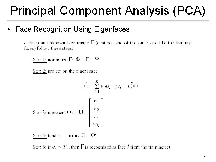
Principal Component Analysis (PCA) • Face Recognition Using Eigenfaces 23

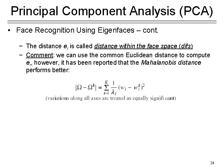
Principal Component Analysis (PCA) • Face Recognition Using Eigenfaces – cont. − The distance er is called distance within the face space (difs) − Comment: we can use the common Euclidean distance to compute er, however, it has been reported that the Mahalanobis distance performs better: 24

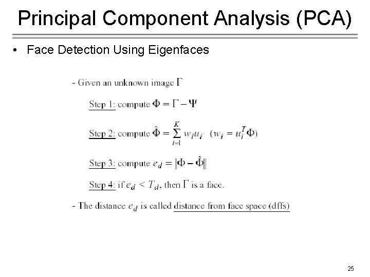
Principal Component Analysis (PCA) • Face Detection Using Eigenfaces 25

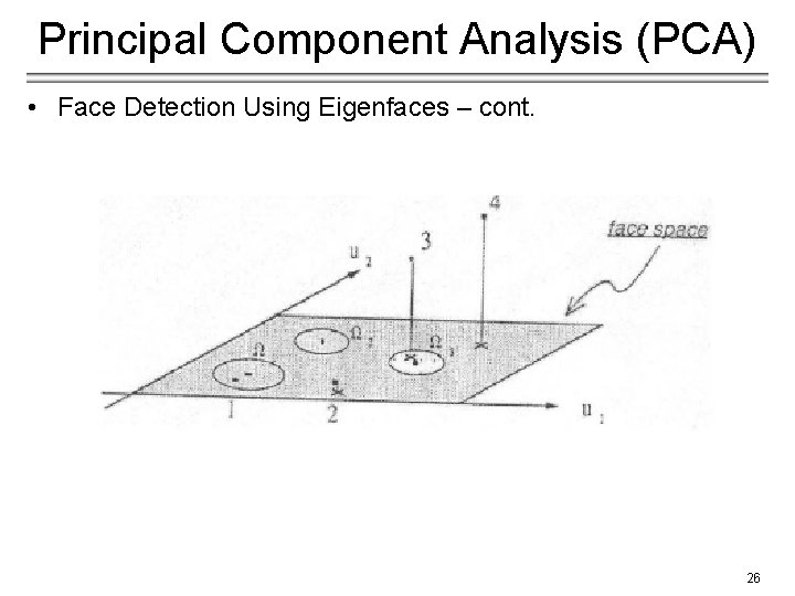
Principal Component Analysis (PCA) • Face Detection Using Eigenfaces – cont. 26

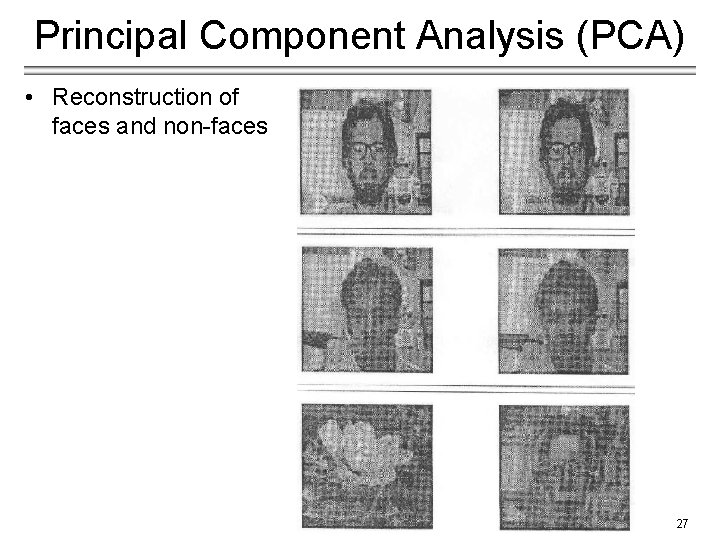
Principal Component Analysis (PCA) • Reconstruction of faces and non-faces 27

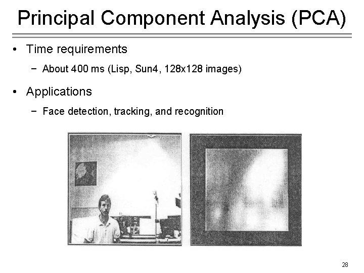
Principal Component Analysis (PCA) • Time requirements − About 400 ms (Lisp, Sun 4, 128 x 128 images) • Applications − Face detection, tracking, and recognition 28

Principal Component Analysis (PCA) • Problems − Background (de-emphasize the outside of the face – e. g. , by multiplying the input image by a 2 D Gaussian window centered on the face) − Lighting conditions (performance degrades with light changes) − Scale (performance decreases quickly with changes to head size) − multi-scale eigenspaces − scale input image to multiple sizes − Orientation (performance decreases but not as fast as with scale changes) − plane rotations can be handled − out-of-plane rotations are more difficult to handle 29

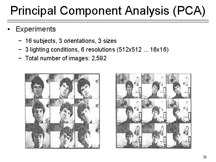
Principal Component Analysis (PCA) • Experiments − 16 subjects, 3 orientations, 3 sizes − 3 lighting conditions, 6 resolutions (512 x 512. . . 16 x 16) − Total number of images: 2, 592 30

Principal Component Analysis (PCA) • Experiment 1 − − − Used various sets of 16 images for training One image/person, taken under the same conditions Eigenfaces were computed offline (7 eigenfaces used) Classify the rest images as one of the 16 individuals No rejections (no threshold for difs) − Performed a large number of experiments and averaged the results: − 96% correct averaged over light variation − 85% correct averaged over orientation variation − 64% correct averaged over size variation 31

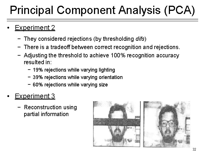
Principal Component Analysis (PCA) • Experiment 2 − They considered rejections (by thresholding difs) − There is a tradeoff between correct recognition and rejections. − Adjusting the threshold to achieve 100% recognition accuracy resulted in: − 19% rejections while varying lighting − 39% rejections while varying orientation − 60% rejections while varying size • Experiment 3 − Reconstruction using partial information 32

Linear Discriminant Analysis (LDA) • Multiple classes and PCA − Suppose there are C classes in the training data. − PCA is based on the sample covariance which characterizes the scatter of the entire data set, irrespective of class-membership. − The projection axes chosen by PCA might not provide good discrimination power. • What is the goal of LDA? − Perform dimensionality reduction while preserving as much of the class discriminatory information as possible. − Seeks to find directions along which the classes are best separated. − Takes into consideration the scatter within-classes but also the scatter between-classes. − More capable of distinguishing image variation due to identity from variation due to other sources such as illumination and expression. 33

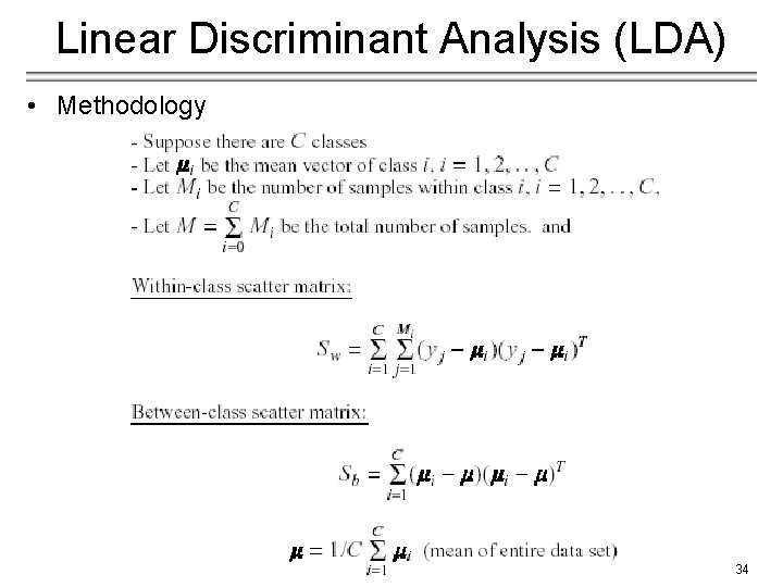
Linear Discriminant Analysis (LDA) • Methodology 34

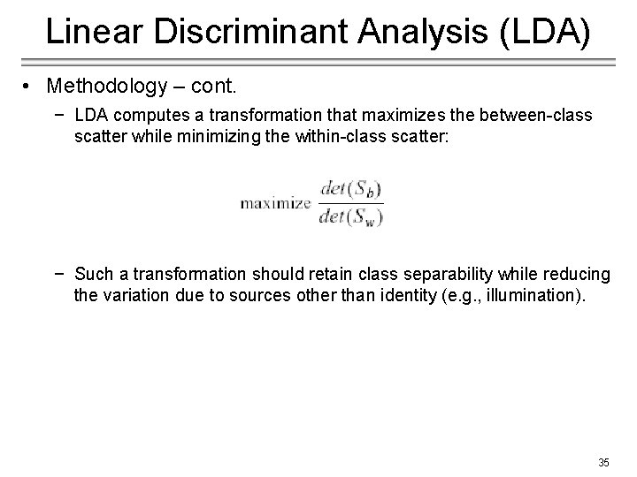
Linear Discriminant Analysis (LDA) • Methodology – cont. − LDA computes a transformation that maximizes the between-class scatter while minimizing the within-class scatter: − Such a transformation should retain class separability while reducing the variation due to sources other than identity (e. g. , illumination). 35

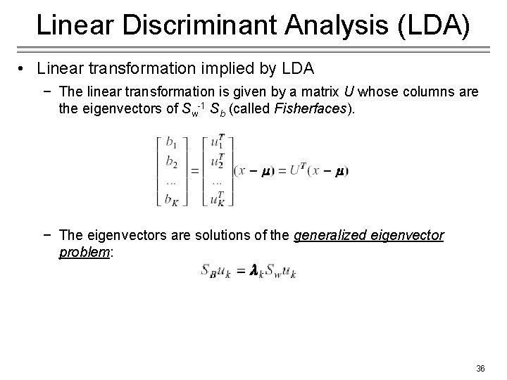
Linear Discriminant Analysis (LDA) • Linear transformation implied by LDA − The linear transformation is given by a matrix U whose columns are the eigenvectors of Sw-1 Sb (called Fisherfaces). − The eigenvectors are solutions of the generalized eigenvector problem: 36

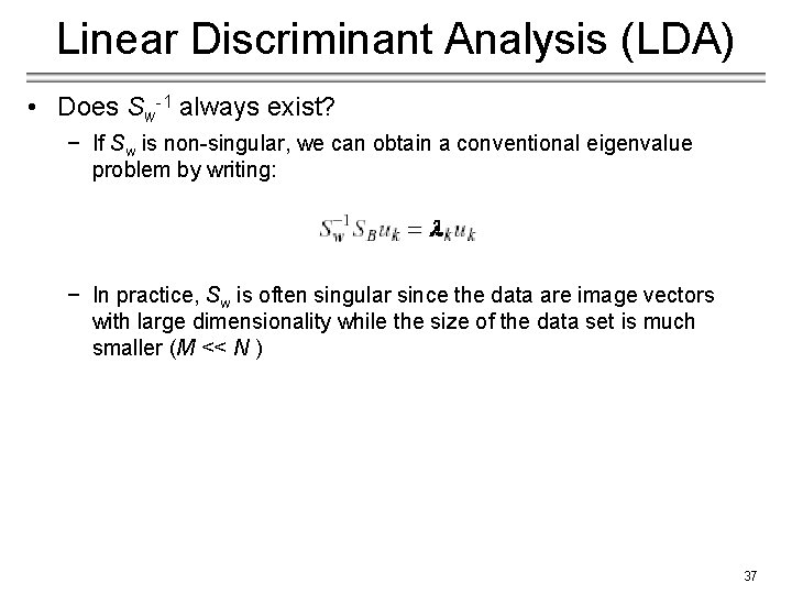
Linear Discriminant Analysis (LDA) • Does Sw-1 always exist? − If Sw is non-singular, we can obtain a conventional eigenvalue problem by writing: − In practice, Sw is often singular since the data are image vectors with large dimensionality while the size of the data set is much smaller (M << N ) 37

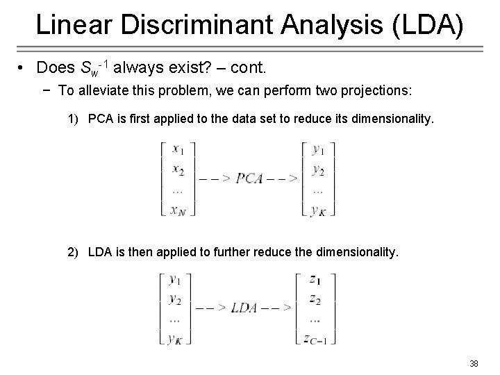
Linear Discriminant Analysis (LDA) • Does Sw-1 always exist? – cont. − To alleviate this problem, we can perform two projections: 1) PCA is first applied to the data set to reduce its dimensionality. 2) LDA is then applied to further reduce the dimensionality. 38

Linear Discriminant Analysis (LDA) • Case Study: Using Discriminant Eigenfeatures for Image Retrieval − D. Swets, J. Weng, "Using Discriminant Eigenfeatures for Image Retrieval", IEEE Transactions on Pattern Analysis and Machine Intelligence, vol. 18, no. 8, pp. 831 -836, 1996. • Content-based image retrieval − The application being studied here is query-by-example image retrieval. − The paper deals with the problem of selecting a good set of image features for content-based image retrieval. 39

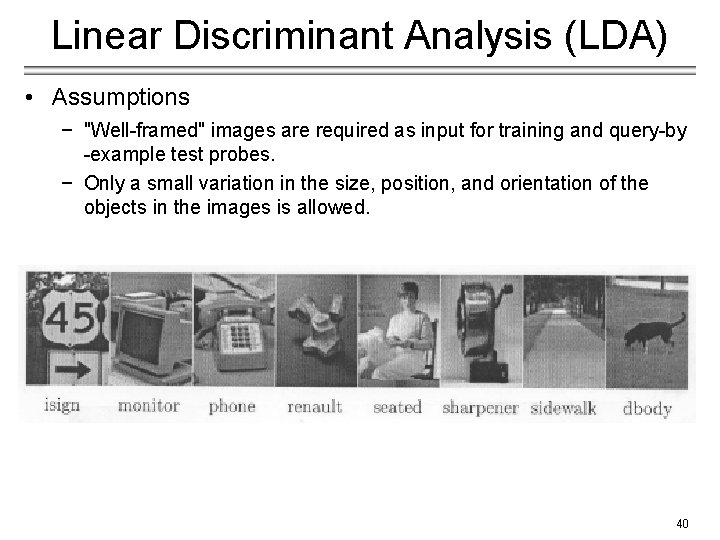
Linear Discriminant Analysis (LDA) • Assumptions − "Well-framed" images are required as input for training and query-by -example test probes. − Only a small variation in the size, position, and orientation of the objects in the images is allowed. 40

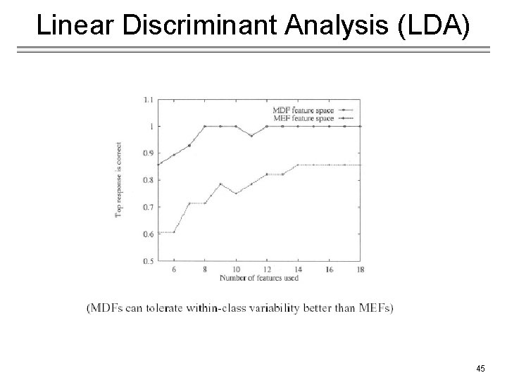
Linear Discriminant Analysis (LDA) • Some terminology − Most Expressive Features (MEF): the features (projections) obtained using PCA. − Most Discriminating Features (MDF): the features (projections) obtained using LDA. • Computational considerations − When computing the eigenvalues/eigenvectors of Sw-1 SBuk = kuk numerically, the computations can be unstable since Sw-1 SB is not always symmetric. − See paper for a way to find the eigenvalues/eigenvectors in a stable way. − Important: Dimensionality of LDA is bounded by C-1 --- this is the rank of Sw-1 SB 41

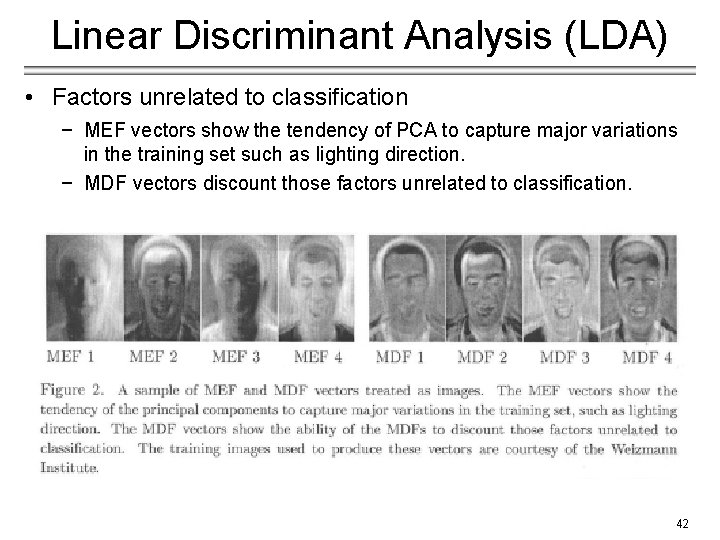
Linear Discriminant Analysis (LDA) • Factors unrelated to classification − MEF vectors show the tendency of PCA to capture major variations in the training set such as lighting direction. − MDF vectors discount those factors unrelated to classification. 42

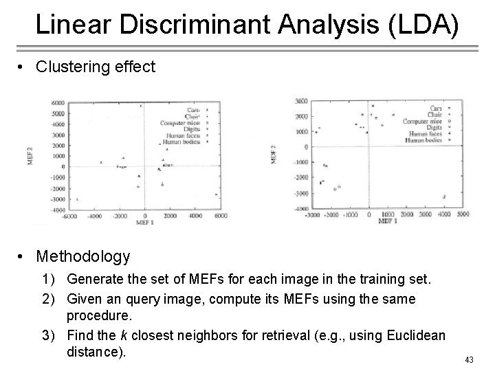
Linear Discriminant Analysis (LDA) • Clustering effect • Methodology 1) Generate the set of MEFs for each image in the training set. 2) Given an query image, compute its MEFs using the same procedure. 3) Find the k closest neighbors for retrieval (e. g. , using Euclidean distance). 43

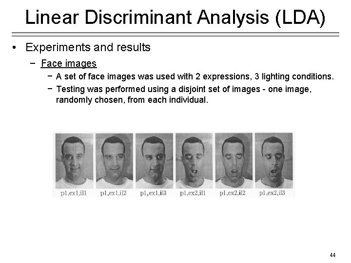
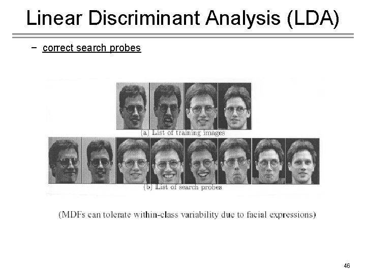
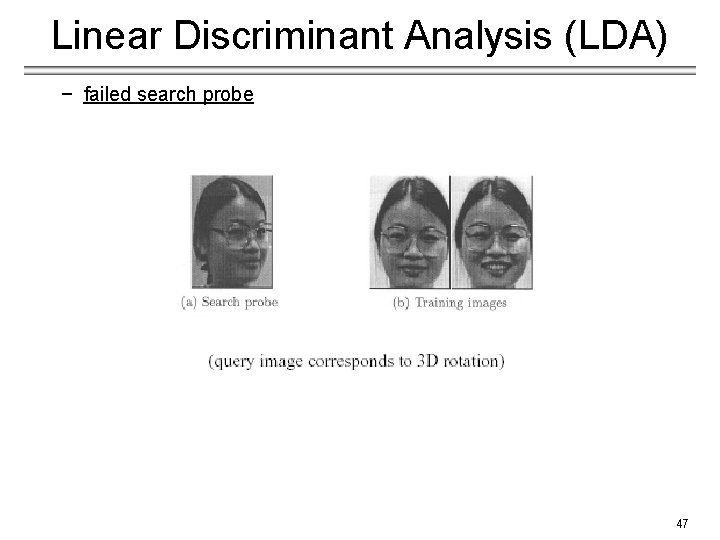
Linear Discriminant Analysis (LDA) • Experiments and results − Face images − A set of face images was used with 2 expressions, 3 lighting conditions. − Testing was performed using a disjoint set of images - one image, randomly chosen, from each individual. 44

Linear Discriminant Analysis (LDA) 45

Linear Discriminant Analysis (LDA) − correct search probes 46

Linear Discriminant Analysis (LDA) − failed search probe 47

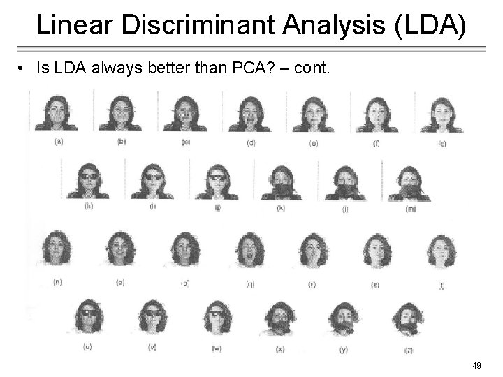
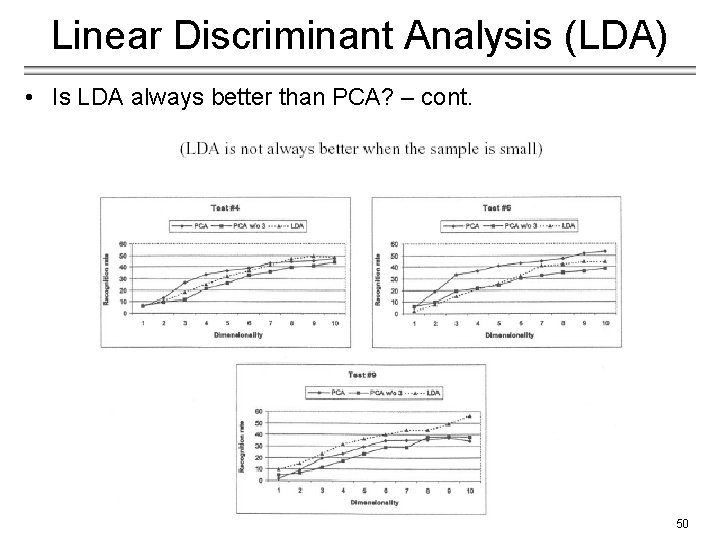
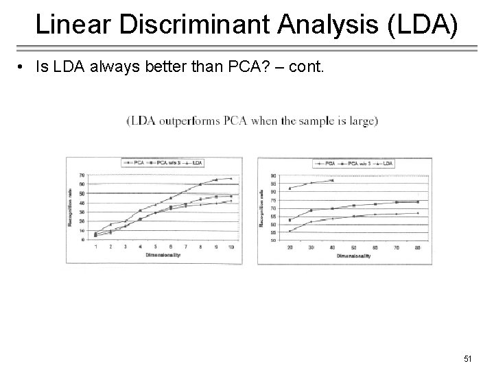
Linear Discriminant Analysis (LDA) • Case Study: PCA versus LDA − A. Martinez, A. Kak, "PCA versus LDA", IEEE Transactions on Pattern Analysis and Machine Intelligence, vol. 23, no. 2, pp. 228233, 2001. • Is LDA always better than PCA? − There has been a tendency in the computer vision community to prefer LDA over PCA. − This is mainly because LDA deals directly with discrimination between classes while PCA does not pay attention to the underlying class structure. − This paper shows that when the training set is small, PCA can outperform LDA. − When the number of samples is large and representative for each class, LDA outperforms PCA. 48

Linear Discriminant Analysis (LDA) • Is LDA always better than PCA? – cont. 49

Linear Discriminant Analysis (LDA) • Is LDA always better than PCA? – cont. 50

Linear Discriminant Analysis (LDA) • Is LDA always better than PCA? – cont. 51

Linear Discriminant Analysis (LDA) • Critique of LDA − Only linearly separable classes will remain separable after applying LDA. − It does not seem to be superior to PCA when the training data set is small. 52