Parallelismo Parallel Cost Execution time sequential Ts parallel

Parallelismo

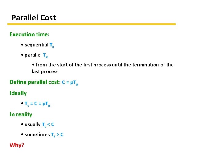
Parallel Cost Execution time: • sequential Ts • parallel Tp • from the start of the first process until the termination of the last process Define parallel cost: C = p. Tp Ideally • Ts = C = p. Tp In reality • usually Ts < C • sometimes Ts > C Why?

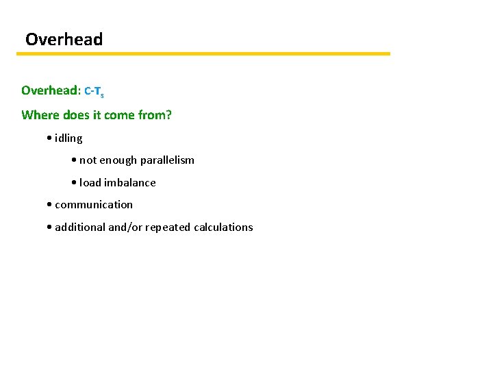
Overhead: C-Ts Where does it come from? • idling • not enough parallelism • load imbalance • communication • additional and/or repeated calculations

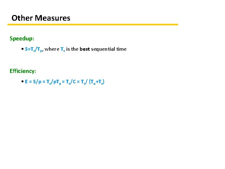
Other Measures Speedup: • S=Ts/Tp, where Ts is the best sequential time Efficiency: • E = S/p = Ts/p. Tp = Ts/C = Ts/ (To+Ts)

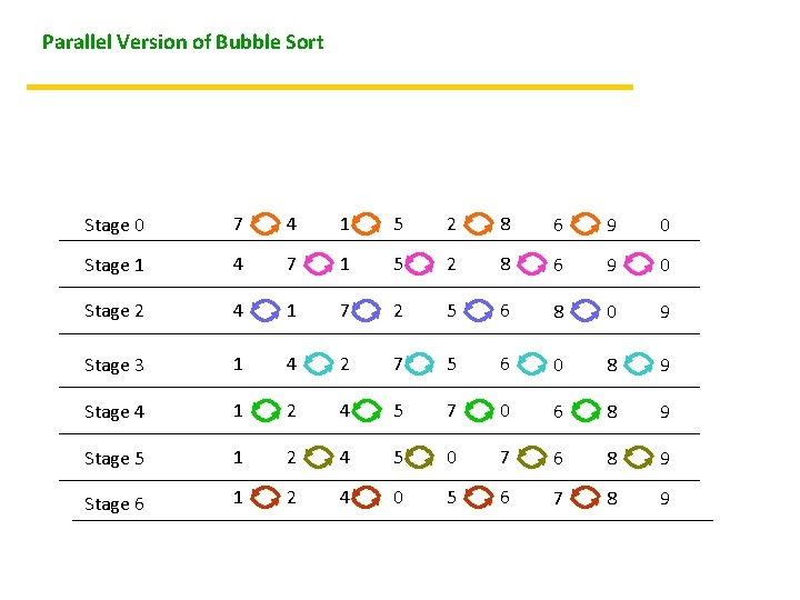
Parallel Version of Bubble Sort Stage 0 7 4 1 5 2 8 6 9 0 Stage 1 4 7 1 5 2 8 6 9 0 Stage 2 4 1 7 2 5 6 8 0 9 Stage 3 1 4 2 7 5 6 0 8 9 Stage 4 1 2 4 5 7 0 6 8 9 Stage 5 1 2 4 5 0 7 6 8 9 Stage 6 1 2 4 0 5 6 7 8 9

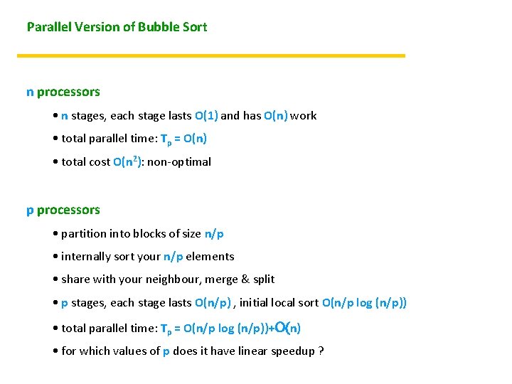
Parallel Version of Bubble Sort n processors • n stages, each stage lasts O(1) and has O(n) work • total parallel time: Tp = O(n) • total cost O(n 2): non-optimal p processors • partition into blocks of size n/p • internally sort your n/p elements • share with your neighbour, merge & split • p stages, each stage lasts O(n/p) , initial local sort O(n/p log (n/p)) • total parallel time: Tp = O(n/p log (n/p))+O(n) • for which values of p does it have linear speedup ?

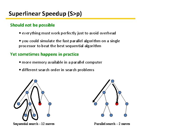
Superlinear Speedup (S>p) Should not be possible • everything must work perfectly just to avoid overhead • you could simulate the fast parallel algorithm on a single processor to beat the best sequential algorithm Yet sometimes happens in practice • more memory available in a parallel computer • different search order in search problems Sequential search – 12 moves Parallel search – 2 moves

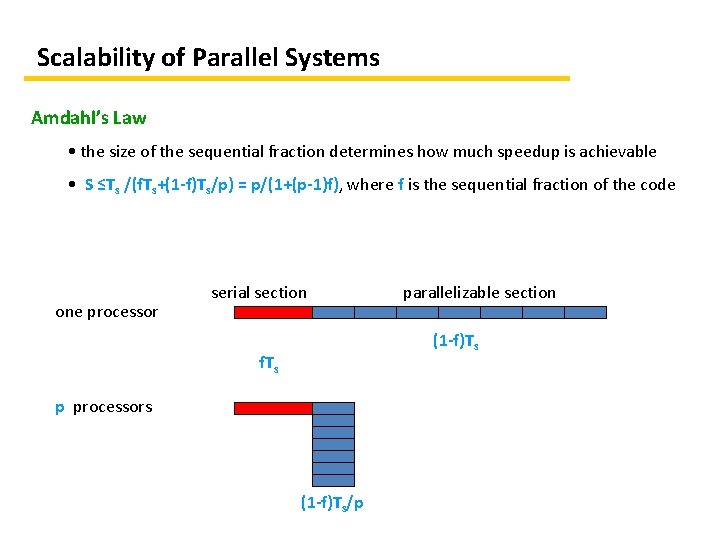
Scalability of Parallel Systems Amdahl’s Law • the size of the sequential fraction determines how much speedup is achievable • S ≤Ts /(f. Ts+(1 -f)Ts/p) = p/(1+(p-1)f), where f is the sequential fraction of the code one processor serial section parallelizable section (1 -f)Ts f. Ts p processors (1 -f)Ts/p

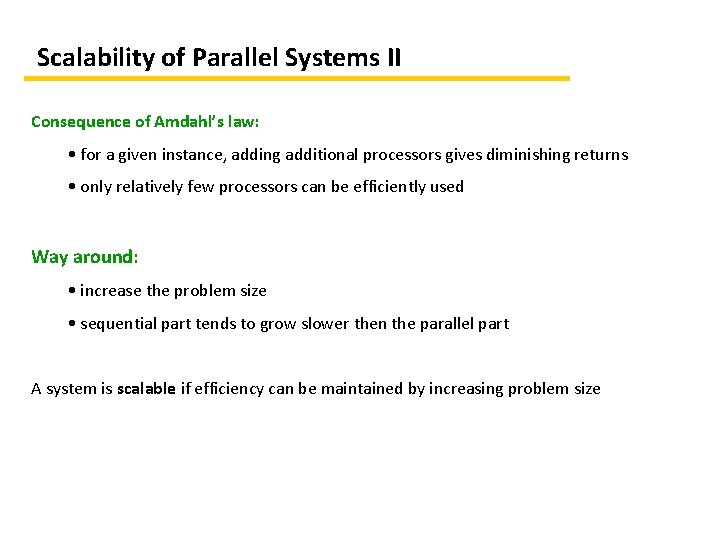
Scalability of Parallel Systems II Consequence of Amdahl’s law: • for a given instance, adding additional processors gives diminishing returns • only relatively few processors can be efficiently used Way around: • increase the problem size • sequential part tends to grow slower then the parallel part A system is scalable if efficiency can be maintained by increasing problem size

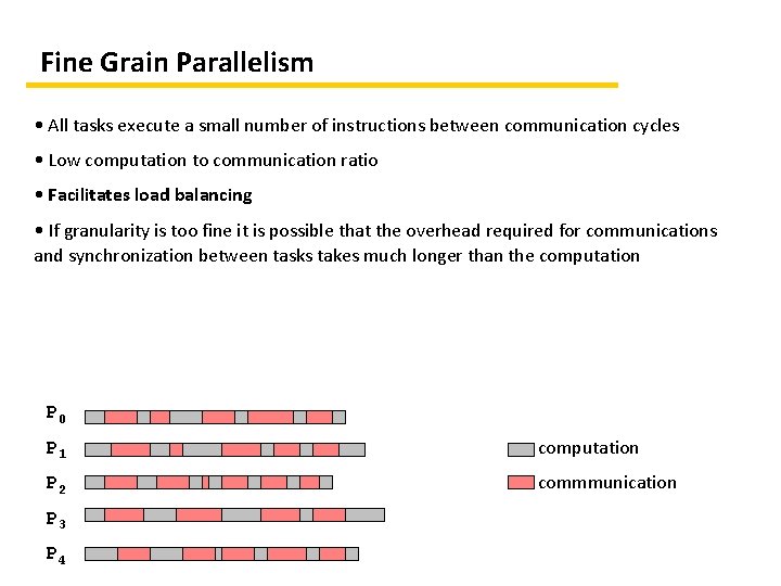
Fine Grain Parallelism • All tasks execute a small number of instructions between communication cycles • Low computation to communication ratio • Facilitates load balancing • If granularity is too fine it is possible that the overhead required for communications and synchronization between tasks takes much longer than the computation P 0 P 1 computation P 2 commmunication P 3 P 4

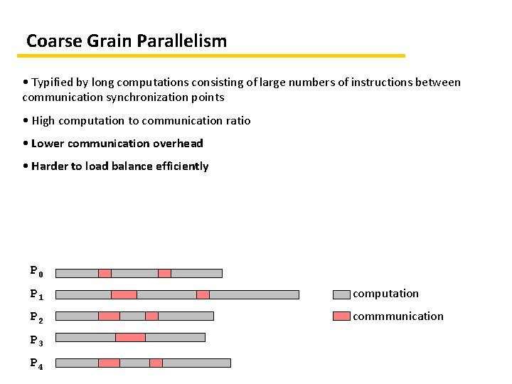
Coarse Grain Parallelism • Typified by long computations consisting of large numbers of instructions between communication synchronization points • High computation to communication ratio • Lower communication overhead • Harder to load balance efficiently P 0 P 1 computation P 2 commmunication P 3 P 4

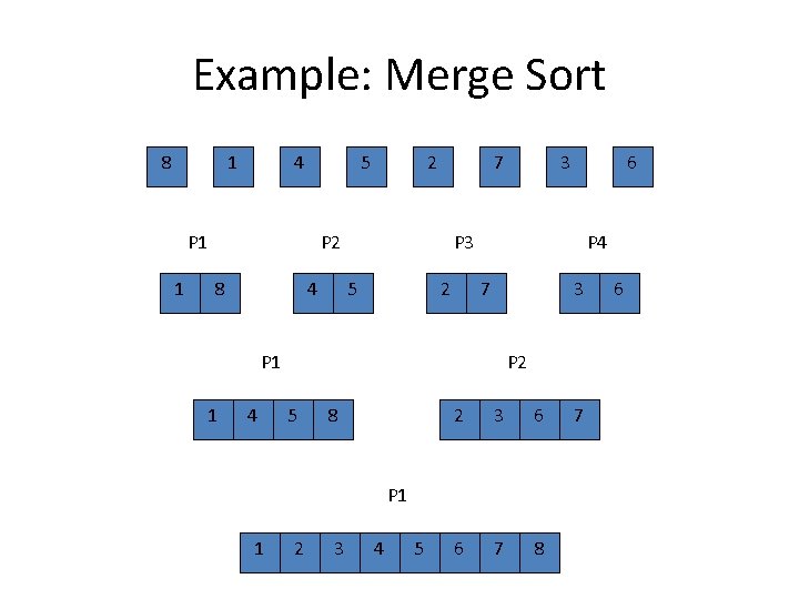
Example: Merge Sort 8 1 4 5 P 1 1 2 7 P 2 8 4 4 5 2 P 4 7 3 P 2 5 8 2 3 6 6 7 8 P 1 1 6 P 3 P 1 1 3 2 3 4 5 7 6

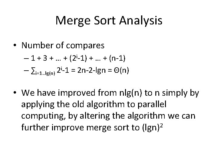
Merge Sort Analysis • Number of compares – 1 + 3 + … + (2 i-1) + … + (n-1) – ∑i=1. . lg(n) 2 i-1 = 2 n-2 -lgn = Θ(n) • We have improved from nlg(n) to n simply by applying the old algorithm to parallel computing, by altering the algorithm we can further improve merge sort to (lgn)2

Parallel Design and Dynamic Programming • Often in a dynamic programming algorithm a given row or diagonal can be computed simultaneously • This makes many dynamic programming algorithms amenable for parallel architectures

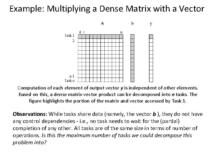
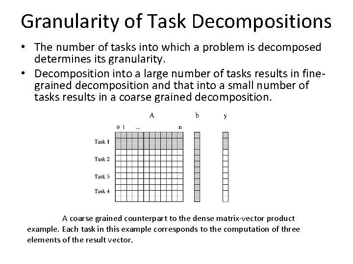
Example: Multiplying a Dense Matrix with a Vector Computation of each element of output vector y is independent of other elements. Based on this, a dense matrix-vector product can be decomposed into n tasks. The figure highlights the portion of the matrix and vector accessed by Task 1. Observations: While tasks share data (namely, the vector b ), they do not have any control dependencies - i. e. , no task needs to wait for the (partial) completion of any other. All tasks are of the same size in terms of number of operations. Is this the maximum number of tasks we could decompose this problem into?

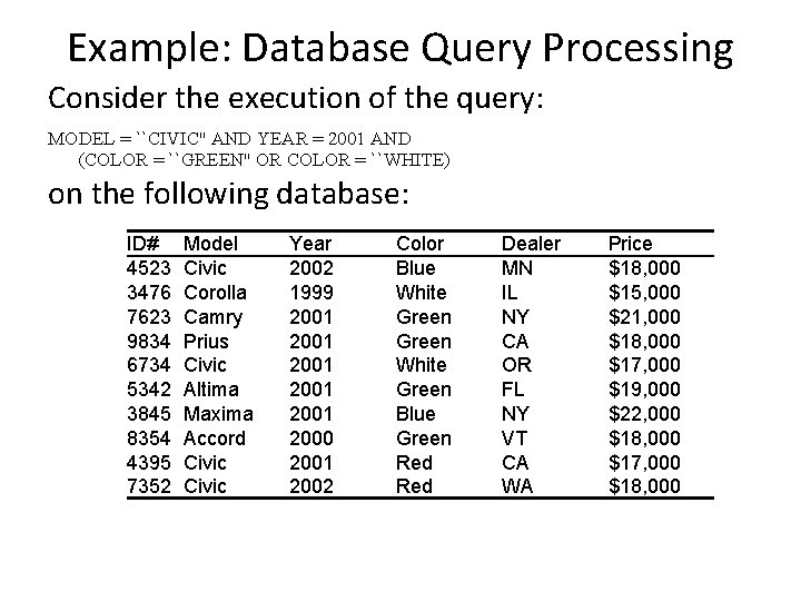
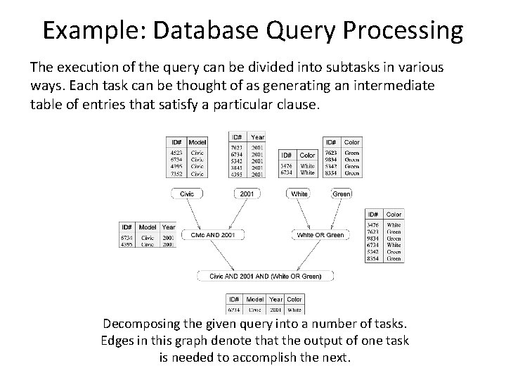
Example: Database Query Processing Consider the execution of the query: MODEL = ``CIVIC'' AND YEAR = 2001 AND (COLOR = ``GREEN'' OR COLOR = ``WHITE) on the following database: ID# 4523 3476 7623 9834 6734 5342 3845 8354 4395 7352 Model Civic Corolla Camry Prius Civic Altima Maxima Accord Civic Year 2002 1999 2001 2001 2000 2001 2002 Color Blue White Green Blue Green Red Dealer MN IL NY CA OR FL NY VT CA WA Price $18, 000 $15, 000 $21, 000 $18, 000 $17, 000 $19, 000 $22, 000 $18, 000 $17, 000 $18, 000

Example: Database Query Processing The execution of the query can be divided into subtasks in various ways. Each task can be thought of as generating an intermediate table of entries that satisfy a particular clause. Decomposing the given query into a number of tasks. Edges in this graph denote that the output of one task is needed to accomplish the next.

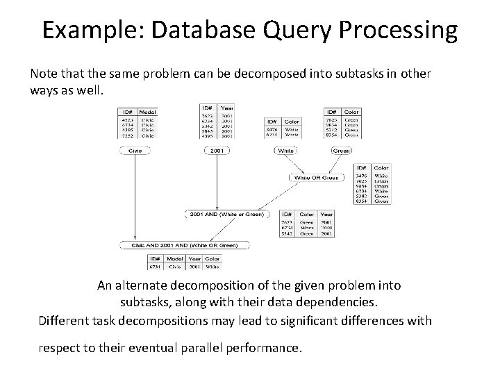
Example: Database Query Processing Note that the same problem can be decomposed into subtasks in other ways as well. An alternate decomposition of the given problem into subtasks, along with their data dependencies. Different task decompositions may lead to significant differences with respect to their eventual parallel performance.

Granularity of Task Decompositions • The number of tasks into which a problem is decomposed determines its granularity. • Decomposition into a large number of tasks results in finegrained decomposition and that into a small number of tasks results in a coarse grained decomposition. A coarse grained counterpart to the dense matrix-vector product example. Each task in this example corresponds to the computation of three elements of the result vector.

Degree of Concurrency • The number of tasks that can be executed in parallel is the degree of concurrency of a decomposition. • Since the number of tasks that can be executed in parallel may change over program execution, the maximum degree of concurrency is the maximum number of such tasks at any point during execution. What is the maximum degree of concurrency of the database query examples? • The average degree of concurrency is the average number of tasks that can be processed in parallel over the execution of the program. Assuming that each tasks in the database example takes identical processing time, what is the average degree of concurrency in each decomposition? • The degree of concurrency increases as the decomposition becomes finer in granularity and vice versa.

Critical Path Length • A directed path in the task dependency graph represents a sequence of tasks that must be processed one after the other. • The longest such path determines the shortest time in which the program can be executed in parallel. • The length of the longest path in a task dependency graph is called the critical path length.

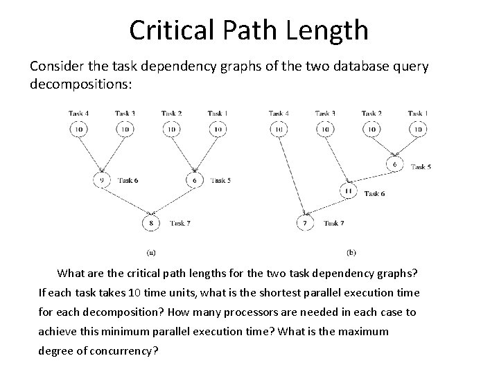
Critical Path Length Consider the task dependency graphs of the two database query decompositions: What are the critical path lengths for the two task dependency graphs? If each task takes 10 time units, what is the shortest parallel execution time for each decomposition? How many processors are needed in each case to achieve this minimum parallel execution time? What is the maximum degree of concurrency?

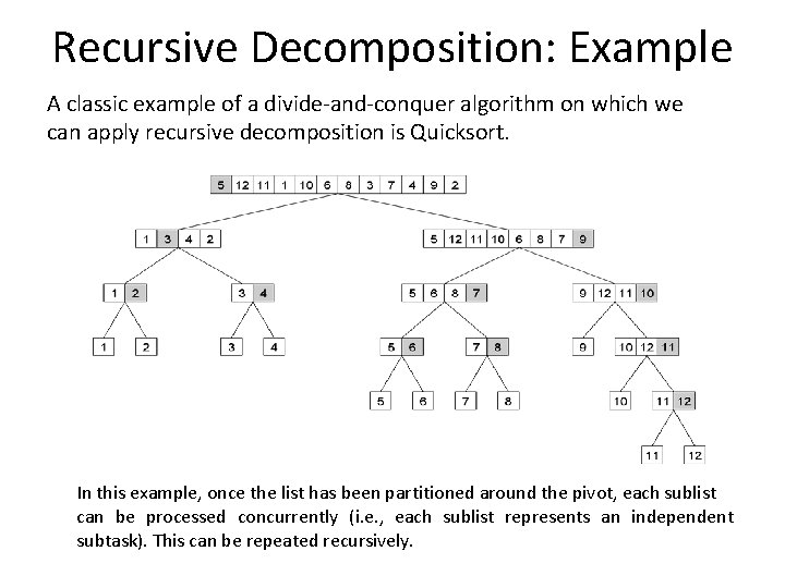
Recursive Decomposition: Example A classic example of a divide-and-conquer algorithm on which we can apply recursive decomposition is Quicksort. In this example, once the list has been partitioned around the pivot, each sublist can be processed concurrently (i. e. , each sublist represents an independent subtask). This can be repeated recursively.

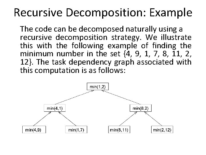
Recursive Decomposition: Example The code can be decomposed naturally using a recursive decomposition strategy. We illustrate this with the following example of finding the minimum number in the set {4, 9, 1, 7, 8, 11, 2, 12}. The task dependency graph associated with this computation is as follows:

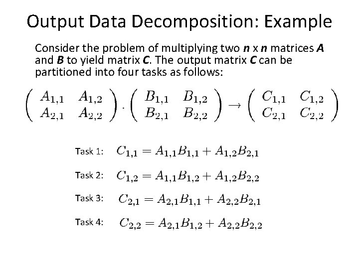
Output Data Decomposition: Example Consider the problem of multiplying two n x n matrices A and B to yield matrix C. The output matrix C can be partitioned into four tasks as follows: Task 1: Task 2: Task 3: Task 4:

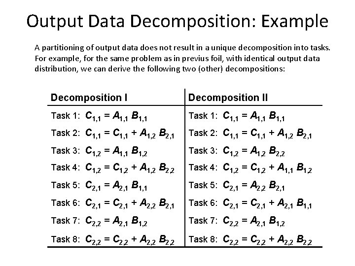
Output Data Decomposition: Example A partitioning of output data does not result in a unique decomposition into tasks. For example, for the same problem as in previus foil, with identical output data distribution, we can derive the following two (other) decompositions: Decomposition II Task 1: C 1, 1 = A 1, 1 B 1, 1 Task 2: C 1, 1 = C 1, 1 + A 1, 2 B 2, 1 Task 3: C 1, 2 = A 1, 1 B 1, 2 Task 3: C 1, 2 = A 1, 2 B 2, 2 Task 4: C 1, 2 = C 1, 2 + A 1, 1 B 1, 2 Task 5: C 2, 1 = A 2, 1 B 1, 1 Task 5: C 2, 1 = A 2, 2 B 2, 1 Task 6: C 2, 1 = C 2, 1 + A 2, 1 B 1, 1 Task 7: C 2, 2 = A 2, 1 B 1, 2 Task 8: C 2, 2 = C 2, 2 + A 2, 2 B 2, 2

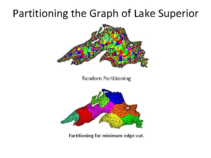
Partitioning the Graph of Lake Superior Random Partitioning for minimum edge-cut.