Optimal Photometry of Faint Galaxies Kenneth M Lanzetta

Optimal Photometry of Faint Galaxies Kenneth M. Lanzetta Stony Brook University

Collaborator: • Stefan Gromoll (Stony Brook University)

Outline • • scientific motivation data photometric redshift technique optimal photometry and photometric redshifts of faint galaxies

Cosmic chemical evolution • We are interested in the quantities of cosmic chemical evolution… – Ωg (damped Ly absorbers) – (rest-frame ultraviolet, H emission) – Z (damped Ly absorbers) – Ωs (rest-frame near-infrared emission) • …which are the quantities of galactic chemical evolution averaged over cosmic volumes

Comoving mass density of gas Compiled by Rao et al. 2005

Comoving star formation rate density Compiled by Lanzetta et al. 2003

Cosmic metallicity Compiled by Prochaska et al. 2004

Outstanding issues • very limited statistics • cosmic variance • selection biases – damped Ly absorbers: obscuration by dust of QSOs behind high-column-density absorbers – ultraviolet emission: dust extinction, cosmological surface brightness dimming

Equations of cosmic chemical evolution

Comoving mass density of stars • existing surveys target very large numbers of galaxies (statistics) across many fields (cosmic variance) • measurement is based upon rest-frame nearinfrared emission (dust extinction) • objective: determine the comoving mass density of stars versus cosmic epoch with the accuracy needed to obtain a statistically meaningful time derivative

Our program • measure optimal photometry (at observed-frame near-ultraviolet through mid-infrared wavelengths) and photometric redshifts of faint galaxies in GOODS and SWIRE surveys • use rest-frame near-infrared luminosities and restframe optical and near-infrared colors to estimate stellar mass densities • construct comoving mass density of stars versus cosmic epoch

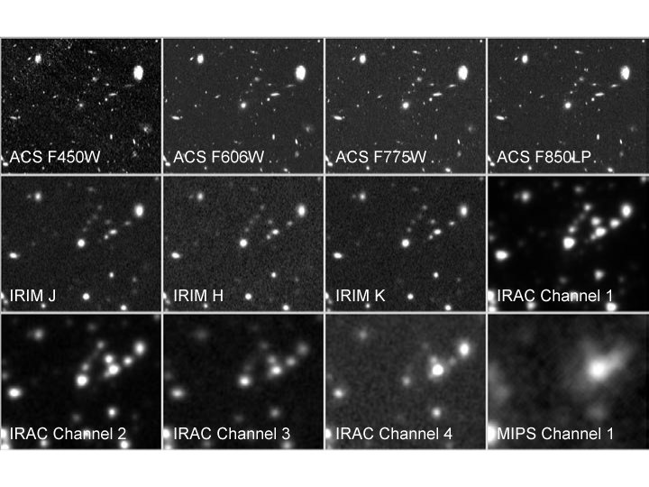
GOODS survey • two fields spanning 320 arcmin 2 • Spitzer IRAC images at 3. 6, 4. 5, 5. 8, and 8. 0 µm and MIPS images at 24 µm • HST and ground-based images at observed-frame optical and near-infrared wavelengths • roughly 10, 000 IRAC images and 10, 000 MIPS images • roughly 200, 000 galaxies at z ≈ 0 – 6

SWIRE survey • six fields spanning 49 deg 2 • Spitzer IRAC images at 3. 6, 4. 5, 5. 8, and 8. 0 µm and MIPS images at 24, 70, and 160 µm • ground-based images at observed-frame optical wavelengths • roughly 100, 000 IRAC images and 500, 000 MIPS images • roughly 8, 000 galaxies at z ≈ 0 – 2

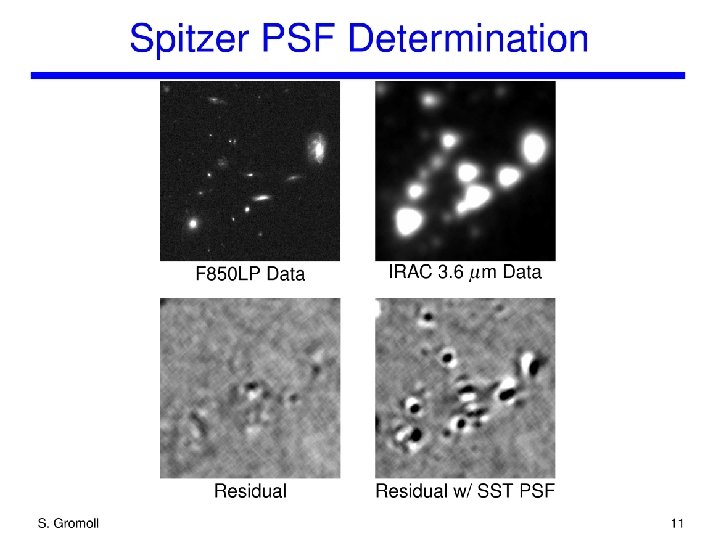
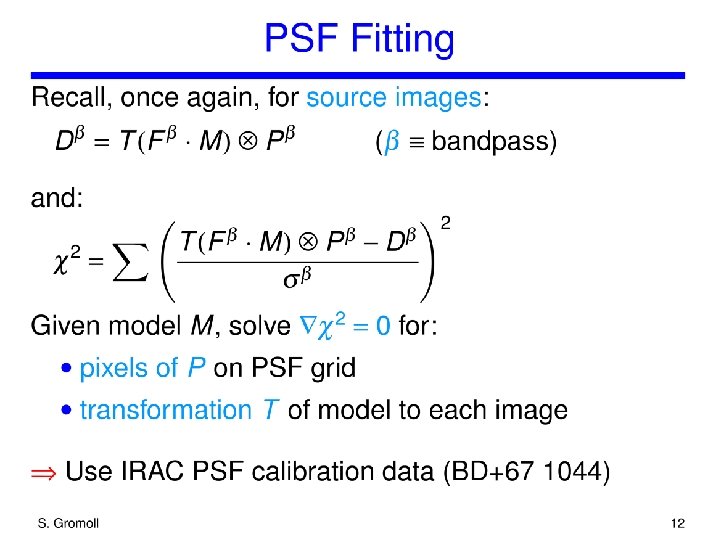
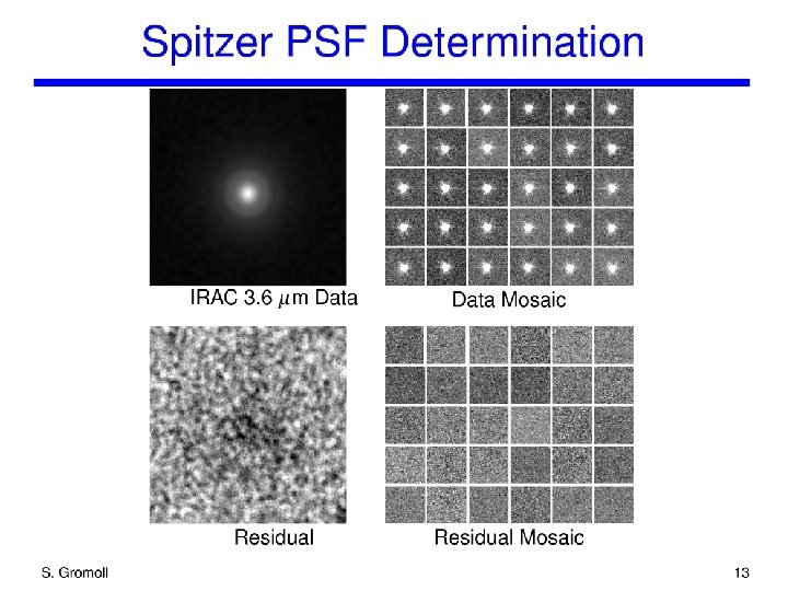
Why the measurement is difficult • characteristic scale of high-redshift galaxies: 0. 1 arcsec • characteristic scale of Spitzer PSF: 2. 5 arcsec (or larger at longer wavelengths) • Spitzer images are undersampled • almost all galaxies overlap other galaxies • how to measure faint galaxies that overlap bright galaxies?

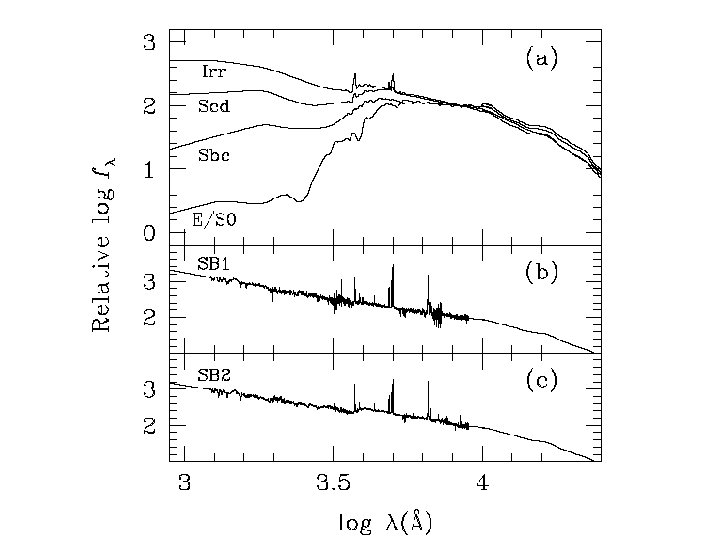
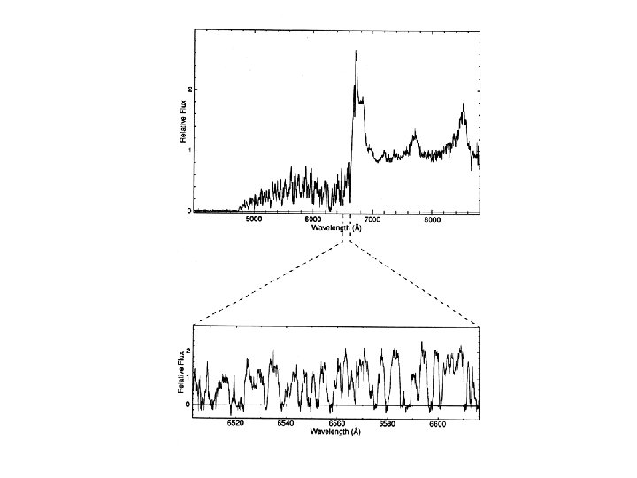
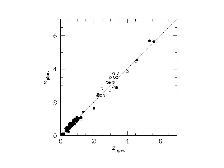
Photometric redshift technique • Determine redshifts by comparing measured and modeled broad-band photometry • Six galaxy spectrophotometric templates • Effects of intrinsic (Lyman limit) and intervening (Lyman-alpha forest and Lyman limit) absorption • Redshift likelihood functions • Demonstrated accurate (∆z / (1 + z) < 6%) and reliable (no outliers) at redshifts z = 0 through 6

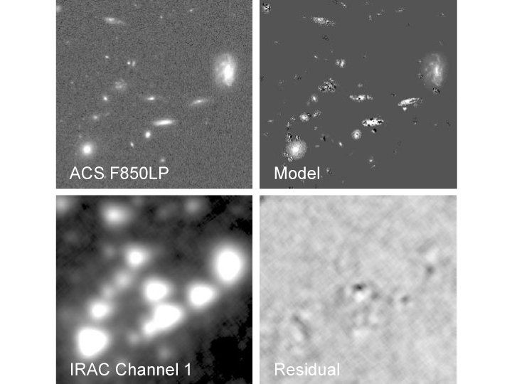
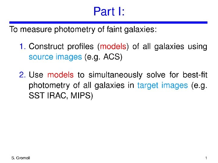
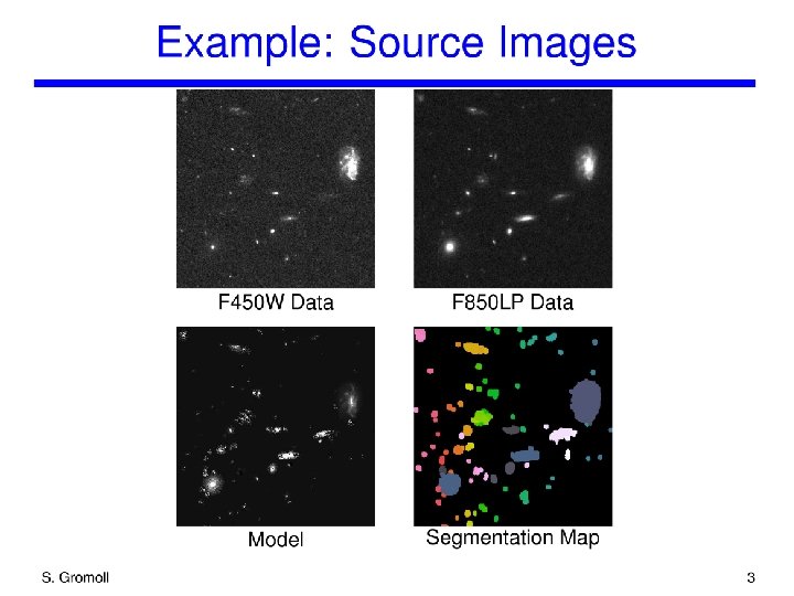
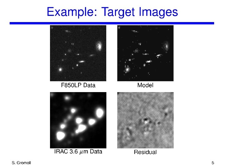
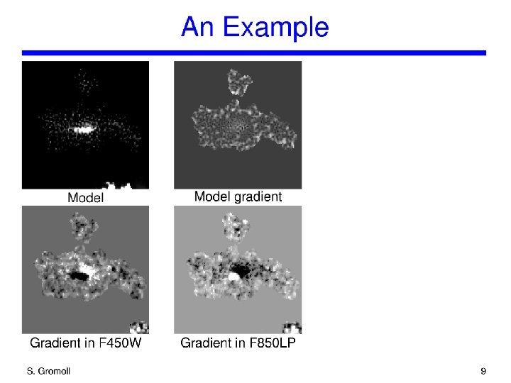
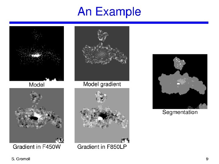
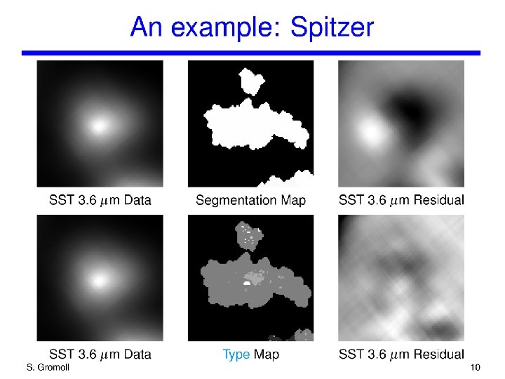
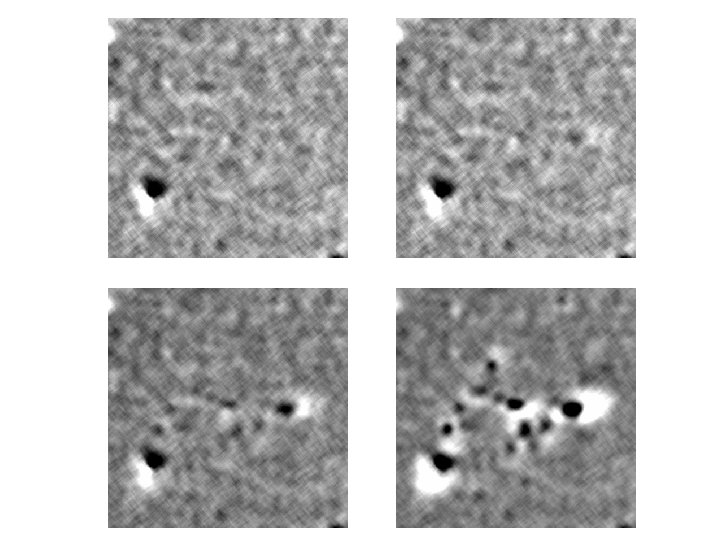
“Redshift spatial profile fitting” technique • “deconvolve” a sequence of “source” images (typically higher-resolution images at optical wavelengths) to obtain photometric redshifts and spatial models of galaxies • use spatial models to fit for energy fluxes in a sequence of “target” images (typically lowerresolution images at near- or mid-infrared wavelengths)

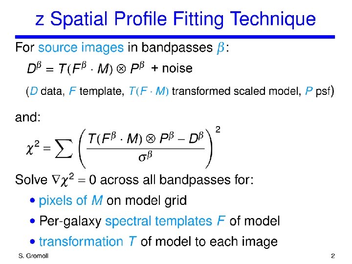
“Deconvolving” source images • build one spatial model image on a fine pixel scale • relate spatial model image to each data image via geometric transformation, convolution, and scaling by spectral templates on a galaxy-by-galaxy basis • simultaneously determine spatial models and photometric redshifts

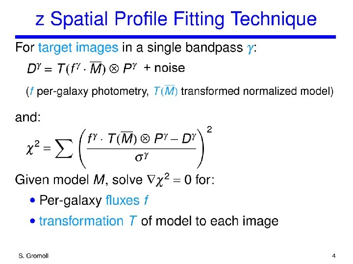
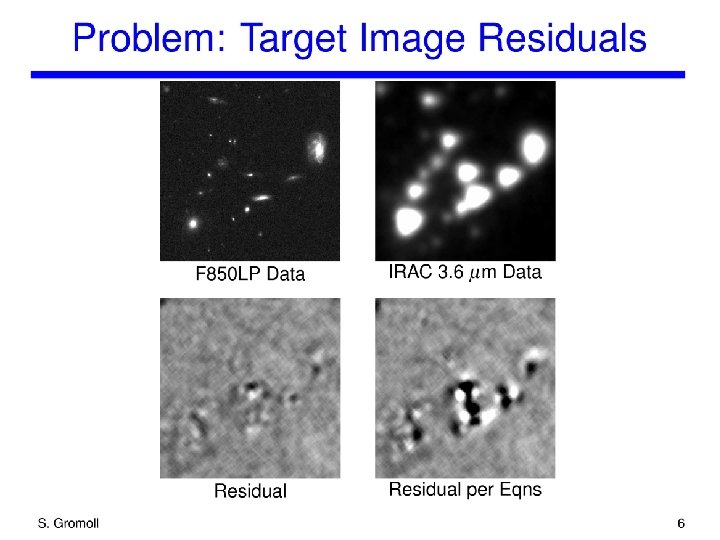
Fitting target images • do not “add” target images (undersampling, correlated noise) • instead, relate spatial model image to each data image via geometric transformation, convolution, and scaling by unknown energy flux on a galaxy-by-galaxy basis • determine energy fluxes

Computational requirement • each step of “deconvolving” or fitting requires transformation and convolution of the spatial model image to each data image • registration of each data image must be fitted for as part of the process • since there a lot of data images, this is computationally very expensive

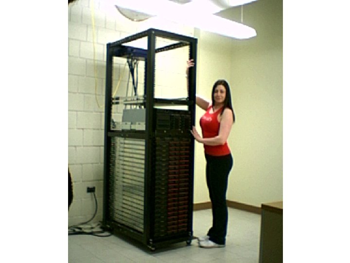
Computer setup • 50 Xeon 3. 06 GHz processors (donated by Intel Corporation) • 20 cluster nodes, four workstations, one file server • two Itanium 1. 4 GHz processors (donated by Ion Computers) • one database server • 2 TB disk storage, 10 TB local disk caches • custom job control and database software

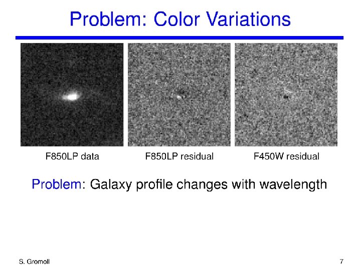
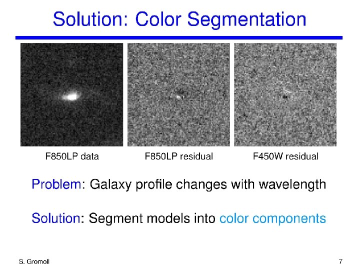
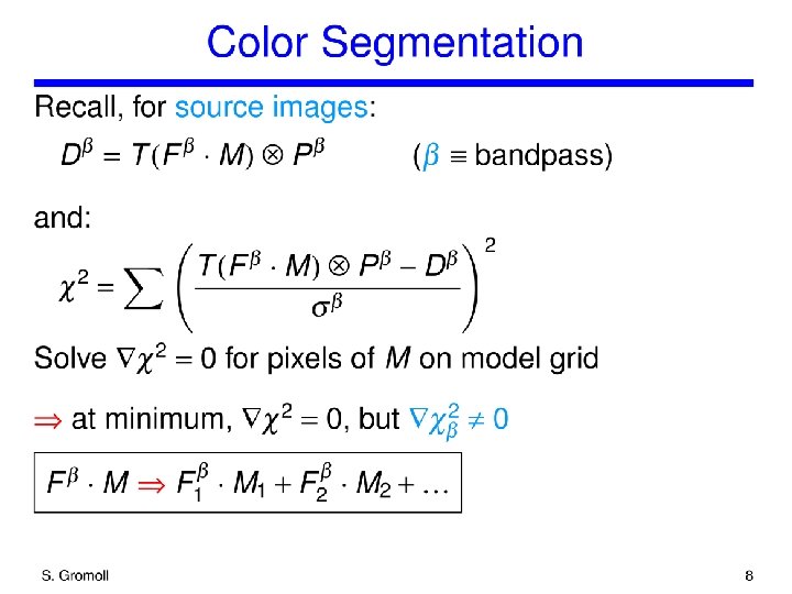
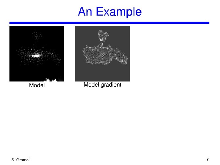
What is needed to measure faint galaxies in deep Spitzer images • accurate image alignment – geometric distortion, registration – better than 0. 01 pixel • accurate spatial models – deconvolution of source images – convolution of target images • “color segmentation” – segment galaxy profiles by color

Image alignment • Geometric distortion and registration––how to calibrate? • S/N = 500 for a typical SST “pixel” • Required image alignment accuracy better than 0. 01 pixel • More or less solved

Noise in source images • S/N = 500 for a typical SST pixel • S/N = 200 over a comparable region of sky for ACS • noise in source images is the limiting systematic effect in measuring SST images • SST images cannot be measured to within noise given current ACS images

Summary • We believe that faint galaxies can be measured in deep Spitzer images only with. . . • . . . accurate spatial models (alignment, deconvolution and convolution, color segmentation). . . • . . . and computational expense