Nonparametric tests in R MannWhitney U Wilcoxon rank

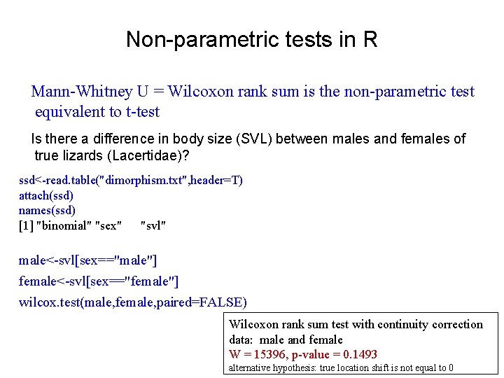
Non-parametric tests in R Mann-Whitney U = Wilcoxon rank sum is the non-parametric test equivalent to t-test Is there a difference in body size (SVL) between males and females of true lizards (Lacertidae)? ssd<-read. table("dimorphism. txt", header=T) attach(ssd) names(ssd) [1] "binomial" "sex" "svl" male<-svl[sex=="male"] female<-svl[sex=="female"] wilcox. test(male, female, paired=FALSE) Wilcoxon rank sum test with continuity correction data: male and female W = 15396, p-value = 0. 1493 alternative hypothesis: true location shift is not equal to 0

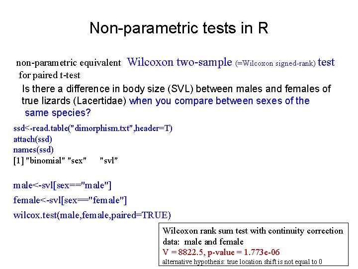
Non-parametric tests in R non-parametric equivalent Wilcoxon two-sample (=Wilcoxon signed-rank) test for paired t-test Is there a difference in body size (SVL) between males and females of true lizards (Lacertidae) when you compare between sexes of the same species? ssd<-read. table("dimorphism. txt", header=T) attach(ssd) names(ssd) [1] "binomial" "sex" "svl" male<-svl[sex=="male"] female<-svl[sex=="female"] wilcox. test(male, female, paired=TRUE) Wilcoxon rank sum test with continuity correction data: male and female V = 8822. 5, p-value = 1. 773 e-06 alternative hypothesis: true location shift is not equal to 0

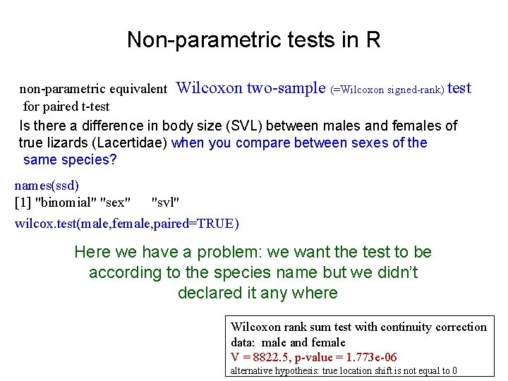
Non-parametric tests in R non-parametric equivalent Wilcoxon two-sample (=Wilcoxon signed-rank) test for paired t-test Is there a difference in body size (SVL) between males and females of true lizards (Lacertidae) when you compare between sexes of the same species? names(ssd) [1] "binomial" "sex" "svl" wilcox. test(male, female, paired=TRUE) Here we have a problem: we want the test to be according to the species name but we didn’t declared it any where Wilcoxon rank sum test with continuity correction data: male and female V = 8822. 5, p-value = 1. 773 e-06 alternative hypothesis: true location shift is not equal to 0

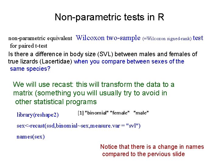
Non-parametric tests in R non-parametric equivalent Wilcoxon two-sample (=Wilcoxon signed-rank) test for paired t-test Is there a difference in body size (SVL) between males and females of true lizards (Lacertidae) when you compare between sexes of the same species? We will use recast: this will transform the data to a matrix (something you will usually try to avoid in other statistical programs library(reshape 2) [1] "binomial" "female" "male" sex<-recast(ssd, binomial~sex, measure. var = "svl") names(sex) Notice that there is a change in names compared to the pervious slide

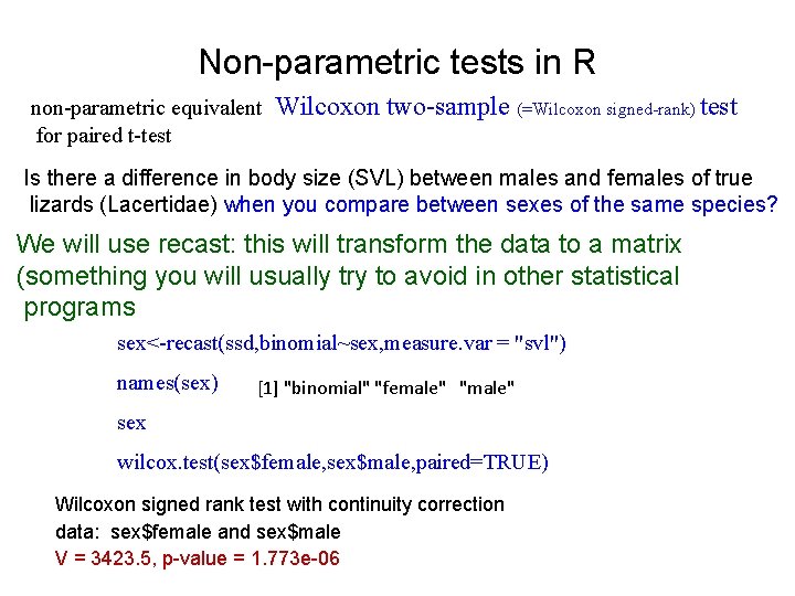
Non-parametric tests in R non-parametric equivalent for paired t-test Wilcoxon two-sample (=Wilcoxon signed-rank) test Is there a difference in body size (SVL) between males and females of true lizards (Lacertidae) when you compare between sexes of the same species? We will use recast: this will transform the data to a matrix (something you will usually try to avoid in other statistical programs sex<-recast(ssd, binomial~sex, measure. var = "svl") names(sex) [1] "binomial" "female" "male" sex wilcox. test(sex$female, sex$male, paired=TRUE) Wilcoxon signed rank test with continuity correction data: sex$female and sex$male V = 3423. 5, p-value = 1. 773 e-06

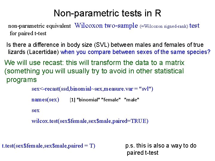
Non-parametric tests in R non-parametric equivalent for paired t-test Wilcoxon two-sample (=Wilcoxon signed-rank) test Is there a difference in body size (SVL) between males and females of true lizards (Lacertidae) when you compare between sexes of the same species? We will use recast: this will transform the data to a matrix (something you will usually try to avoid in other statistical programs sex<-recast(ssd, binomial~sex, measure. var = "svl") names(sex) [1] "binomial" "female" "male" sex wilcox. test(sex$female, sex$male, paired=TRUE) t. test(sex$female, sex$male, paired = T) p. s. this is also a way to do paired t-test

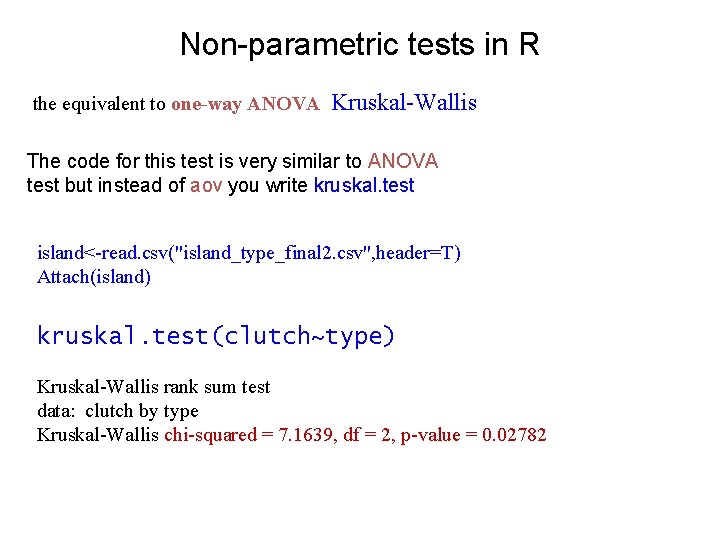
Non-parametric tests in R the equivalent to one-way ANOVA Kruskal-Wallis The code for this test is very similar to ANOVA test but instead of aov you write kruskal. test island<-read. csv("island_type_final 2. csv", header=T) Attach(island) kruskal. test(clutch~type) Kruskal-Wallis rank sum test data: clutch by type Kruskal-Wallis chi-squared = 7. 1639, df = 2, p-value = 0. 02782

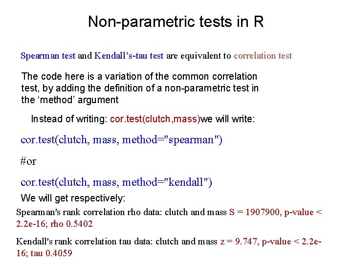
Non-parametric tests in R Spearman test and Kendall’s-tau test are equivalent to correlation test The code here is a variation of the common correlation test, by adding the definition of a non-parametric test in the ‘method’ argument Instead of writing: cor. test(clutch, mass)we will write: cor. test(clutch, mass, method="spearman") #or cor. test(clutch, mass, method="kendall") We will get respectively: Spearman's rank correlation rho data: clutch and mass S = 1907900, p-value < 2. 2 e-16; rho 0. 5402 Kendall's rank correlation tau data: clutch and mass z = 9. 747, p-value < 2. 2 e 16; tau 0. 4059

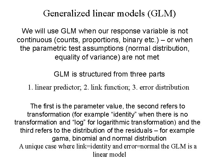
Generalized linear models (GLM) We will use GLM when our response variable is not continuous (counts, proportions, binary etc. ) – or when the parametric test assumptions (normal distribution, equality of variance) are not met GLM is structured from three parts 1. linear predictor; 2. link function; 3. error distribution The first is the parameter value, the second refers to transformation (for example “identity” when there is no transformation and “log” for logarithmic transformation) and the third refers to the distribution of the residuals – for example gama, binomial and normal distribution A unique case where link=identity and error=normal the GLM is a linear model

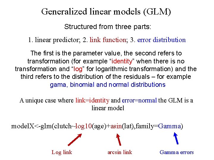
Generalized linear models (GLM) Structured from three parts: 1. linear predictor; 2. link function; 3. error distribution The first is the parameter value, the second refers to transformation (for example “identity” when there is no transformation and “log” for logarithmic transformation) and the third refers to the distribution of the residuals – for example gama, binomial and normal distributions A unique case where link=identity and error=normal the GLM is a linear model. X<-glm(clutch~log 10(age)+asin(lat), family=Gamma) Log link arcsin link Gamma errors

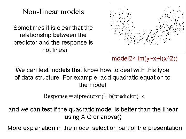
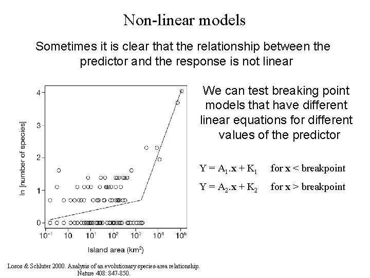
Non-linear models Sometimes it is clear that the relationship between the predictor and the response is not linear model 2<-lm(y~x+I(x^2)) We can test models that know how to deal with this type of data structure. For example: add quadratic equation to the model Response = a(predictor)2+b(predictor)+c and we can test if the quadratic model is better than the linear using AIC or anova() More explanation in the model selection part of the presentation

Non-linear models Sometimes it is clear that the relationship between the predictor and the response is not linear We can test breaking point models that have different linear equations for different values of the predictor Y = A 1. x + K 1 for x < breakpoint Y = A 2. x + K 2 for x > breakpoint Losos & Schluter 2000. Analysis of an evolutionary species-area relationship. Nature 408: 847 -850.

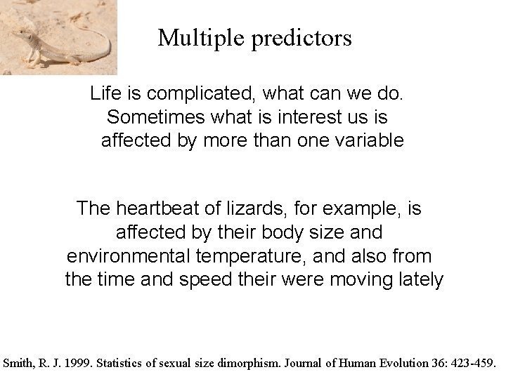
Multiple predictors Life is complicated, what can we do. Sometimes what is interest us is affected by more than one variable The heartbeat of lizards, for example, is affected by their body size and environmental temperature, and also from the time and speed their were moving lately Smith, R. J. 1999. Statistics of sexual size dimorphism. Journal of Human Evolution 36: 423 -459.

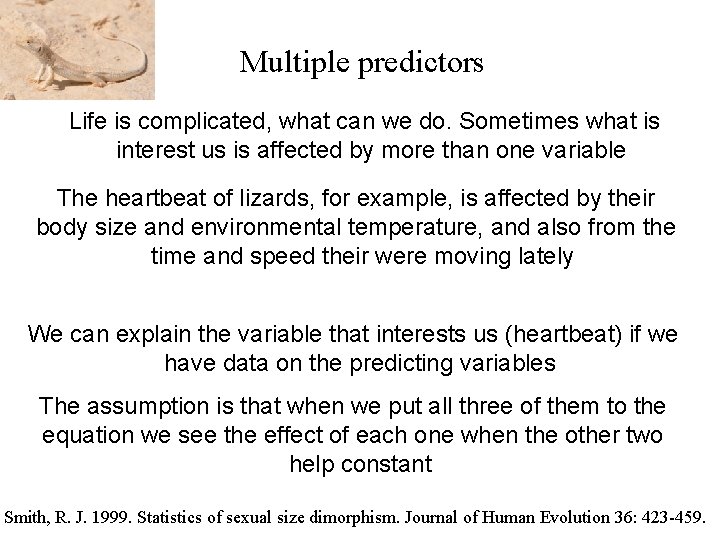
Multiple predictors Life is complicated, what can we do. Sometimes what is interest us is affected by more than one variable The heartbeat of lizards, for example, is affected by their body size and environmental temperature, and also from the time and speed their were moving lately We can explain the variable that interests us (heartbeat) if we have data on the predicting variables The assumption is that when we put all three of them to the equation we see the effect of each one when the other two help constant Smith, R. J. 1999. Statistics of sexual size dimorphism. Journal of Human Evolution 36: 423 -459.

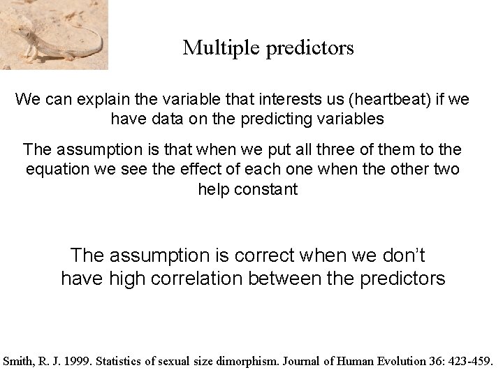
Multiple predictors We can explain the variable that interests us (heartbeat) if we have data on the predicting variables The assumption is that when we put all three of them to the equation we see the effect of each one when the other two help constant The assumption is correct when we don’t have high correlation between the predictors Smith, R. J. 1999. Statistics of sexual size dimorphism. Journal of Human Evolution 36: 423 -459.

Which test should we choose? If we have a few predictor variable (lets say 4) and they are all categorical the test for them will be ANOVA (lets say 4 -way ANOVA) If we have a few predictor variables (lets say seven) and they are all continuous the test for them will be Multiple Regression

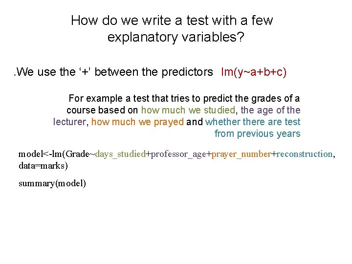
How do we write a test with a few explanatory variables? . We use the ‘+’ between the predictors lm(y~a+b+c) For example a test that tries to predict the grades of a course based on how much we studied, the age of the lecturer, how much we prayed and whethere are test from previous years model<-lm(Grade~days_studied+professor_age+prayer_number+reconstruction, data=marks) summary(model)

Which test should we choose? If we have a few predictor variables (at least 2) – part of them (at least one) are categorical and part of them (at least one) are continuous the test for them will be ANCOVA (analysis of co-variance)

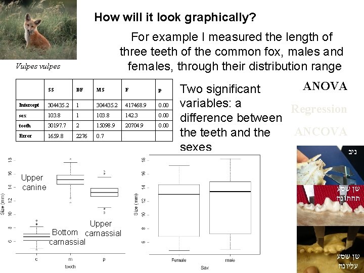
How will it look graphically? For example I measured the length of three teeth of the common fox, males and females, through their distribution range Vulpes vulpes SS DF MS F p Intercept 304435. 2 1 304435. 2 417468. 9 0. 00 sex 103. 8 142. 3 0. 00 tooth 30197. 7 2 15098. 9 20704. 9 0. 00 Error 1659. 8 2276 0. 7 Upper canine ANOVA Two significant variables: a Regression difference between ANCOVA the teeth and the sexes ניב שן שסע תחתונה Upper Bottom carnassial שן שסע עליונה

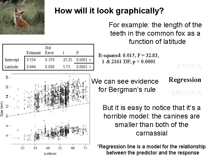
How will it look graphically? For example: the length of the teeth in the common fox as a function of latitude Estimate Std. Error t P Intercept 9. 554 0. 378 25. 25 0. 0001 < Latitude 0. 044 0. 008 5. 73 0. 0001 < R-squared: 0. 015, F = 32. 83, 1 & 2161 DF; p < 0. 0001 We can see evidence for Bergman’s rule ANOVA Regression ANCOVA But it is easy to notice that it’s a horrible model: the canines are smaller than both of the carnassial *Regression line is a model for the relationship between the predictor and the response

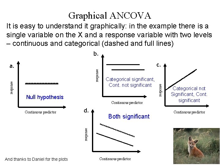
Graphical ANCOVA It is easy to understand it graphically: in the example there is a single variable on the X and a response variable with two levels – continuous and categorical (dashed and full lines) b. response Categorical significant, Cont. not significant Null hypothesis Continuous predictor d. Both significant response Continuous predictor And thanks to Daniel for the plots Continuous predictor response c. a. Categorical not Significant, Cont. significant Continuous predictor

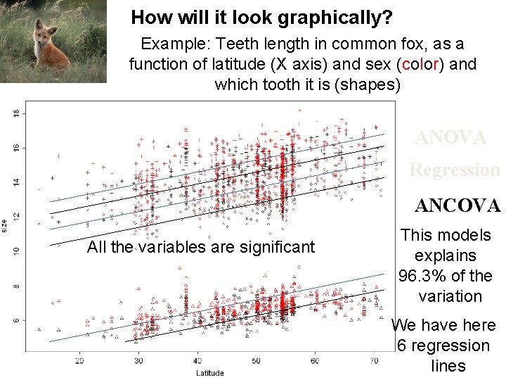
How will it look graphically? Example: Teeth length in common fox, as a function of latitude (X axis) and sex (color) and which tooth it is (shapes) factor Df SS MS F p sex 1 99 99 191. 7 0. 0001 < tooth 2 Latitude 1 436. 1 Residuals 2158 1114. 2 0. 5 28665. 3 14332. 7 27758. 79 0. 0001 < 844. 69 0. 0001 < ANOVA Regression ANCOVA All the variables are significant This models explains 96. 3% of the variation We have here 6 regression lines

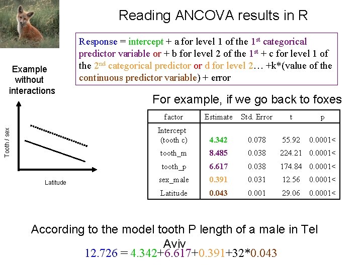
Reading ANCOVA results in R Tooth / sex Example without interactions Latitude Response = intercept + a for level 1 of the 1 st categorical predictor variable or + b for level 2 of the 1 st + c for level 1 of the 2 nd categorical predictor or d for level 2… +k*(value of the continuous predictor variable) + error For example, if we go back to foxes factor Estimate Std. Error t p Intercept (tooth c) 4. 342 0. 078 55. 92 0. 0001< tooth_m 8. 485 0. 038 224. 21 0. 0001< tooth_p 6. 617 0. 038 174. 84 0. 0001< sex_male 0. 391 0. 031 12. 56 0. 0001< Latitude 0. 043 0. 001 29. 06 0. 0001< According to the model tooth P length of a male in Tel Aviv 12. 726 = 4. 342+6. 617+0. 391+32*0. 043

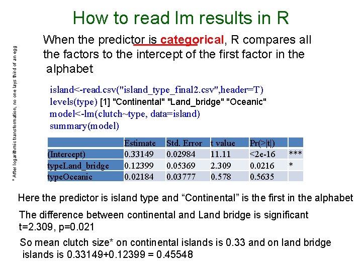
* After logarithmic transformation, no one lays third of an egg How to read lm results in R When the predictor is categorical, R compares all the factors to the intercept of the first factor in the alphabet island<-read. csv("island_type_final 2. csv", header=T) levels(type) [1] "Continental" "Land_bridge" "Oceanic" model<-lm(clutch~type, data=island) summary(model) (Intercept) type. Land_bridge type. Oceanic Estimate 0. 33149 0. 12399 0. 02184 Std. Error 0. 02984 0. 05369 0. 03777 t value 11. 11 2. 309 0. 578 Pr(>|t|) <2 e-16 0. 0216 0. 5635 *** * Here the predictor is island type and “Continental” is the first in the alphabet The difference between continental and Land bridge is significant t=2. 309, p=0. 021 So mean clutch size* on continental islands is 0. 33 and on land bridge islands is 0. 33149+0. 12399 = 0. 45548

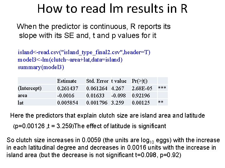
How to read lm results in R When the predictor is continuous, R reports its slope with its SE and, t and p values for it island<-read. csv("island_type_final 2. csv", header=T) model 3<-lm(clutch~area+lat, data=island) summary(model 3) (Intercept) area lat Estimate 0. 261437 -0. 0016 0. 005854 Std. Error 0. 061264 0. 01633 0. 001796 t value 4. 267 -0. 098 3. 259 Pr(>|t|) 2. 68 E-05 *** 0. 92196 0. 00125 ** Here the predictors that explain clutch size are island area and latitude (p=0. 00126 , t = 3. 259)The effect of latitude is significant So clutch size increases in 0. 0059 (the units are log 10 eggs) with the increase in each latitudinal degree and decreases in 0. 0016 units with the increase in island area (but the decrease is not significant t=0. 098, p=0. 92)

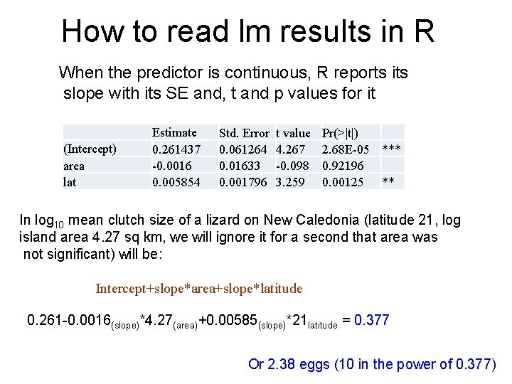
How to read lm results in R When the predictor is continuous, R reports its slope with its SE and, t and p values for it (Intercept) area lat Estimate 0. 261437 -0. 0016 0. 005854 Std. Error 0. 061264 0. 01633 0. 001796 t value 4. 267 -0. 098 3. 259 Pr(>|t|) 2. 68 E-05 *** 0. 92196 0. 00125 ** In log 10 mean clutch size of a lizard on New Caledonia (latitude 21, log island area 4. 27 sq km, we will ignore it for a second that area was not significant) will be: Intercept+slope*area+slope*latitude 0. 261 -0. 0016(slope)*4. 27(area)+0. 00585(slope)*21 latitude = 0. 377 Or 2. 38 eggs (10 in the power of 0. 377)

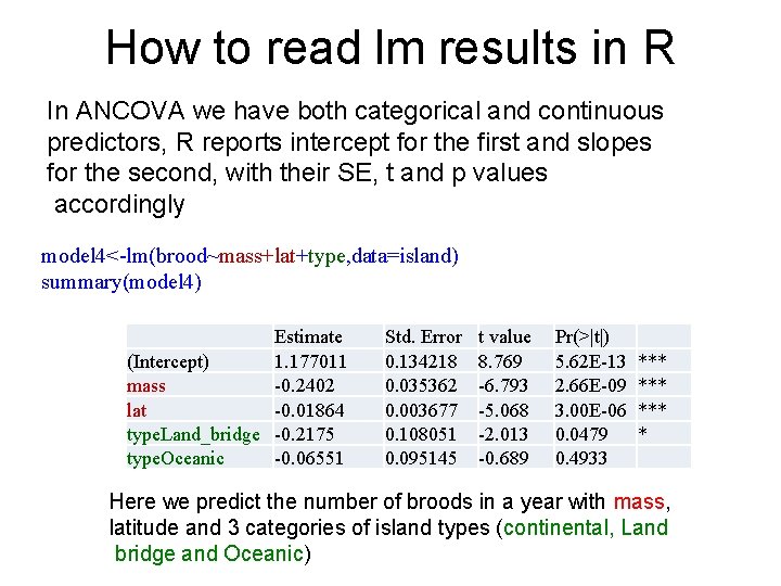
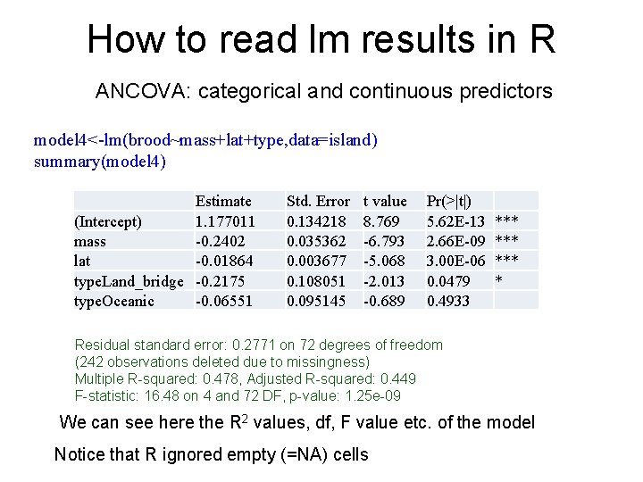
How to read lm results in R In ANCOVA we have both categorical and continuous predictors, R reports intercept for the first and slopes for the second, with their SE, t and p values accordingly model 4<-lm(brood~mass+lat+type, data=island) summary(model 4) Estimate (Intercept) 1. 177011 mass -0. 2402 lat -0. 01864 type. Land_bridge -0. 2175 type. Oceanic -0. 06551 Std. Error 0. 134218 0. 035362 0. 003677 0. 108051 0. 095145 t value 8. 769 -6. 793 -5. 068 -2. 013 -0. 689 Pr(>|t|) 5. 62 E-13 2. 66 E-09 3. 00 E-06 0. 0479 0. 4933 *** *** * Here we predict the number of broods in a year with mass, latitude and 3 categories of island types (continental, Land bridge and Oceanic)

How to read lm results in R ANCOVA: categorical and continuous predictors model 4<-lm(brood~mass+lat+type, data=island) summary(model 4) Estimate (Intercept) 1. 177011 mass -0. 2402 lat -0. 01864 type. Land_bridge -0. 2175 type. Oceanic -0. 06551 Std. Error 0. 134218 0. 035362 0. 003677 0. 108051 0. 095145 t value 8. 769 -6. 793 -5. 068 -2. 013 -0. 689 Pr(>|t|) 5. 62 E-13 2. 66 E-09 3. 00 E-06 0. 0479 0. 4933 *** *** * Residual standard error: 0. 2771 on 72 degrees of freedom (242 observations deleted due to missingness) Multiple R-squared: 0. 478, Adjusted R-squared: 0. 449 F-statistic: 16. 48 on 4 and 72 DF, p-value: 1. 25 e-09 We can see here the R 2 values, df, F value etc. of the model Notice that R ignored empty (=NA) cells

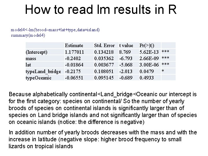
How to read lm results in R model 4<-lm(brood~mass+lat+type, data=island) summary(model 4) Estimate (Intercept) 1. 177011 mass -0. 2402 lat -0. 01864 type. Land_bridge -0. 2175 type. Oceanic -0. 06551 Std. Error 0. 134218 0. 035362 0. 003677 0. 108051 0. 095145 t value 8. 769 -6. 793 -5. 068 -2. 013 -0. 689 Pr(>|t|) 5. 62 E-13 2. 66 E-09 3. 00 E-06 0. 0479 0. 4933 *** *** * Because alphabetically continental<Land_bridge<Oceanic our intercept is for the first category: species on continental/ So the number of yearly broods of species on continental islands is significantly larger than of species on Land bridge islands and not significantly larger than of species on oceanic islands (notice: the difference is negative) In addition number of yearly broods decreases with the mass and with the increase in latitude (negative slope: higher brood frequency to small lizards on tropical islands

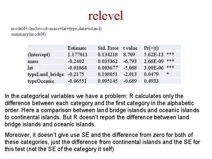
relevel model 4<-lm(brood~mass+lat+type, data=island) summary(model 4) Estimate (Intercept) 1. 177011 mass -0. 2402 lat -0. 01864 type. Land_bridge -0. 2175 type. Oceanic -0. 06551 Std. Error 0. 134218 0. 035362 0. 003677 0. 108051 0. 095145 t value 8. 769 -6. 793 -5. 068 -2. 013 -0. 689 Pr(>|t|) 5. 62 E-13 2. 66 E-09 3. 00 E-06 0. 0479 0. 4933 *** *** * In the categorical variables we have a problem: R calculates only the difference between each category and the first category in the alphabetic order. Here a comparison between land bridge islands and oceanic islands to continental islands. But R doesn’t report the difference between land bridge islands and oceanic islands. Moreover, it doesn’t give use SE and the difference from zero for both of these categories, just the difference from continental islands and the SE for this test (not the SE of the category it self)

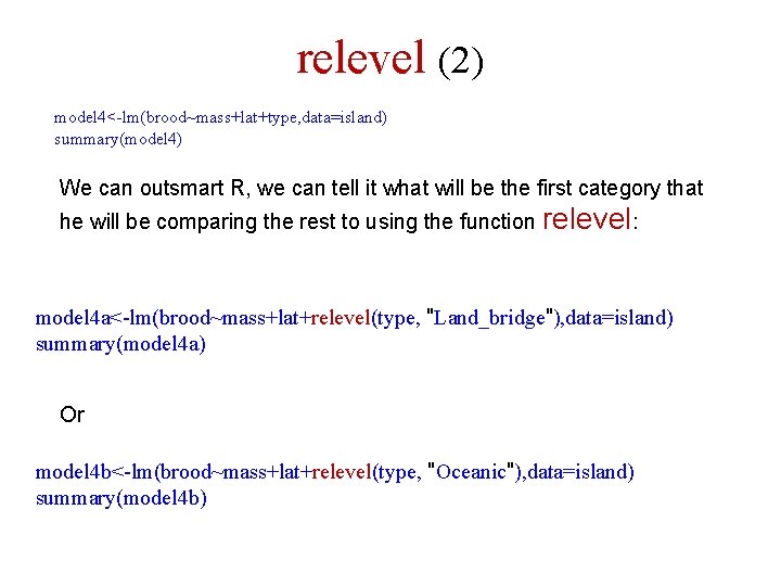
relevel (2) model 4<-lm(brood~mass+lat+type, data=island) summary(model 4) We can outsmart R, we can tell it what will be the first category that he will be comparing the rest to using the function relevel: model 4 a<-lm(brood~mass+lat+relevel(type, "Land_bridge"), data=island) summary(model 4 a) Or model 4 b<-lm(brood~mass+lat+relevel(type, "Oceanic"), data=island) summary(model 4 b)

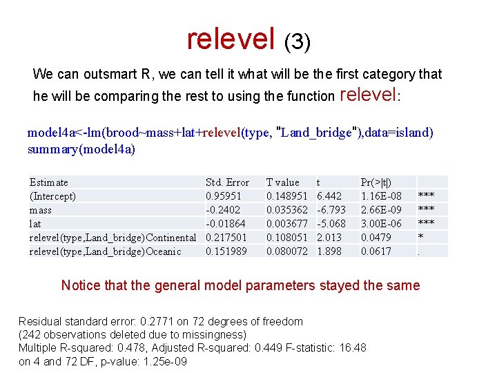
relevel (3) We can outsmart R, we can tell it what will be the first category that he will be comparing the rest to using the function relevel: model 4 a<-lm(brood~mass+lat+relevel(type, "Land_bridge"), data=island) summary(model 4 a) Estimate (Intercept) mass lat relevel(type, Land_bridge)Continental relevel(type, Land_bridge)Oceanic Std. Error 0. 95951 -0. 2402 -0. 01864 0. 217501 0. 151989 T value 0. 148951 0. 035362 0. 003677 0. 108051 0. 080072 t 6. 442 -6. 793 -5. 068 2. 013 1. 898 Pr(>|t|) 1. 16 E-08 2. 66 E-09 3. 00 E-06 0. 0479 0. 0617 *** *** *. Notice that the general model parameters stayed the same Residual standard error: 0. 2771 on 72 degrees of freedom (242 observations deleted due to missingness) Multiple R-squared: 0. 478, Adjusted R-squared: 0. 449 F-statistic: 16. 48 on 4 and 72 DF, p-value: 1. 25 e-09

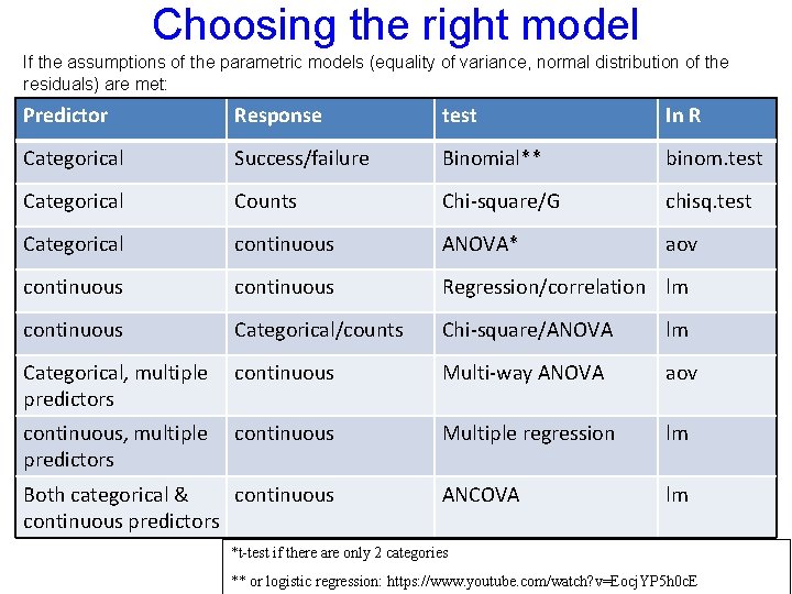
Choosing the right model If the assumptions of the parametric models (equality of variance, normal distribution of the residuals) are met: Predictor Response test In R Categorical Success/failure Binomial** binom. test Categorical Counts Chi-square/G chisq. test Categorical continuous ANOVA* aov continuous Regression/correlation lm continuous Categorical/counts Chi-square/ANOVA lm Categorical, multiple predictors continuous Multi-way ANOVA aov continuous, multiple predictors continuous Multiple regression lm ANCOVA lm Both categorical & continuous predictors *t-test if there are only 2 categories ** or logistic regression: https: //www. youtube. com/watch? v=Eocj. YP 5 h 0 c. E

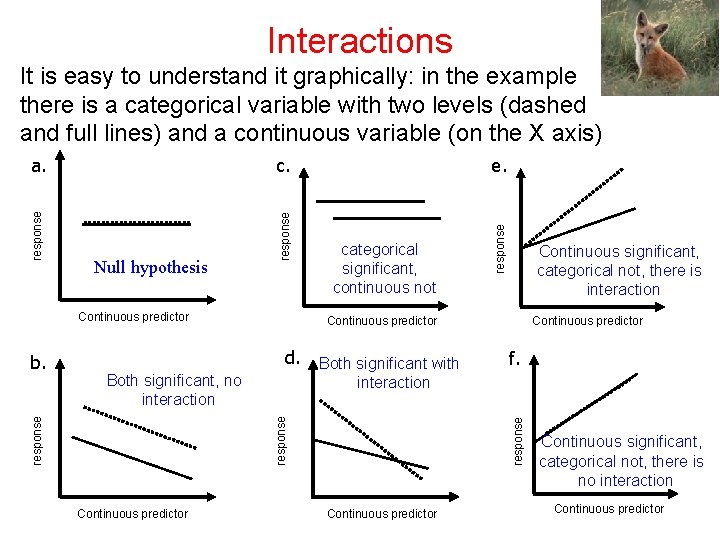
Interactions c. response Null hypothesis Continuous predictor categorical significant, continuous not Both significant with interaction Continuous predictor f. response Both significant, no interaction Continuous predictor Continuous significant, categorical not, there is interaction Continuous predictor d. response b. e. response a. response It is easy to understand it graphically: in the example there is a categorical variable with two levels (dashed and full lines) and a continuous variable (on the X axis) Continuous predictor Continuous significant, categorical not, there is no interaction Continuous predictor

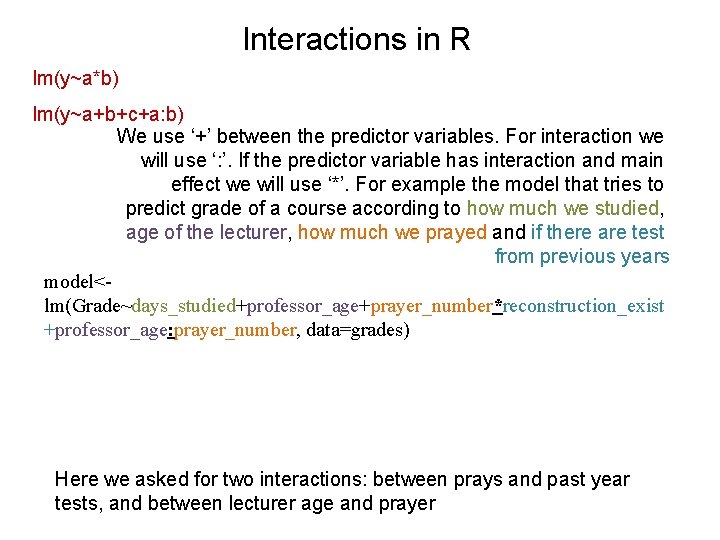
Interactions in R lm(y~a*b) lm(y~a+b+c+a: b) We use ‘+’ between the predictor variables. For interaction we will use ‘: ’. If the predictor variable has interaction and main effect we will use ‘*’. For example the model that tries to predict grade of a course according to how much we studied, age of the lecturer, how much we prayed and if there are test from previous years model<lm(Grade~days_studied+professor_age+prayer_number*reconstruction_exist +professor_age: prayer_number, data=grades) Here we asked for two interactions: between prays and past year tests, and between lecturer age and prayer

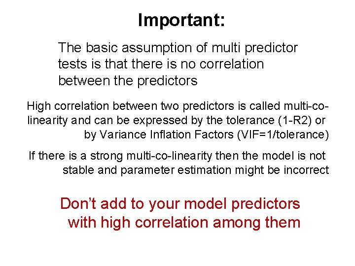
Important: The basic assumption of multi predictor tests is that there is no correlation between the predictors High correlation between two predictors is called multi-colinearity and can be expressed by the tolerance (1 -R 2) or by Variance Inflation Factors (VIF=1/tolerance) If there is a strong multi-co-linearity then the model is not stable and parameter estimation might be incorrect Don’t add to your model predictors with high correlation among them

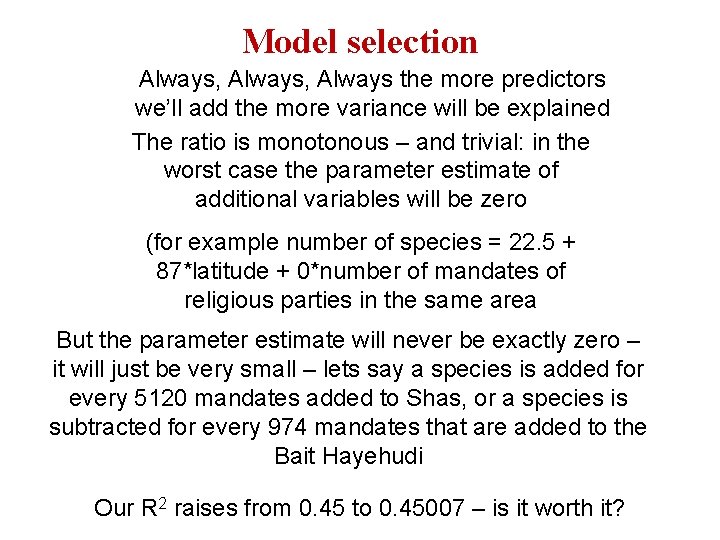
Model selection Always, Always the more predictors we’ll add the more variance will be explained The ratio is monotonous – and trivial: in the worst case the parameter estimate of additional variables will be zero (for example number of species = 22. 5 + 87*latitude + 0*number of mandates of religious parties in the same area But the parameter estimate will never be exactly zero – it will just be very small – lets say a species is added for every 5120 mandates added to Shas, or a species is subtracted for every 974 mandates that are added to the Bait Hayehudi Our R 2 raises from 0. 45 to 0. 45007 – is it worth it?

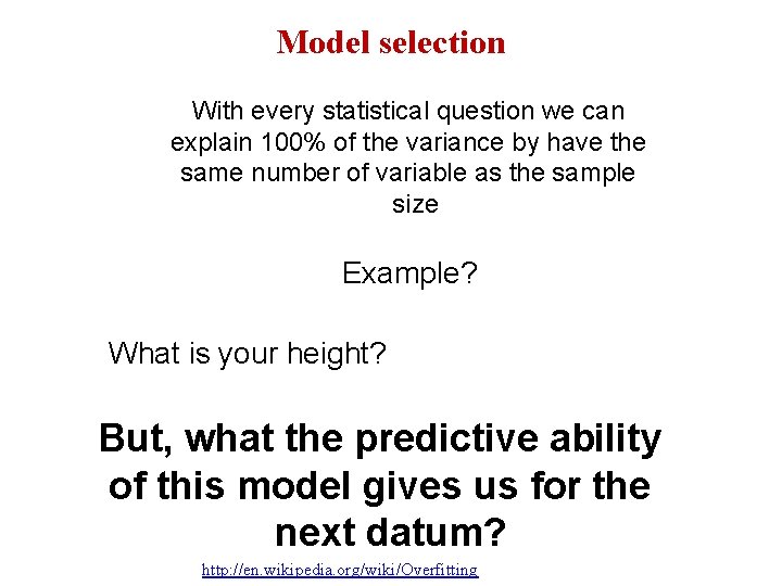
Model selection With every statistical question we can explain 100% of the variance by have the same number of variable as the sample size Example? What is your height? But, what the predictive ability of this model gives us for the next datum? http: //en. wikipedia. org/wiki/Overfitting

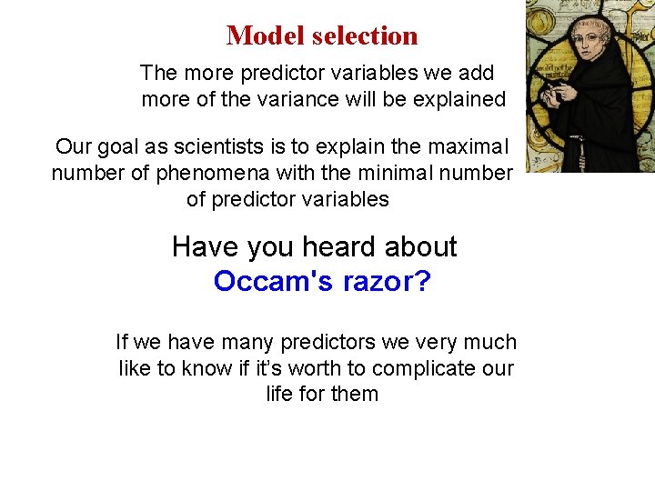
Model selection The more predictor variables we add more of the variance will be explained Our goal as scientists is to explain the maximal number of phenomena with the minimal number of predictor variables Have you heard about Occam's razor? If we have many predictors we very much like to know if it’s worth to complicate our life for them

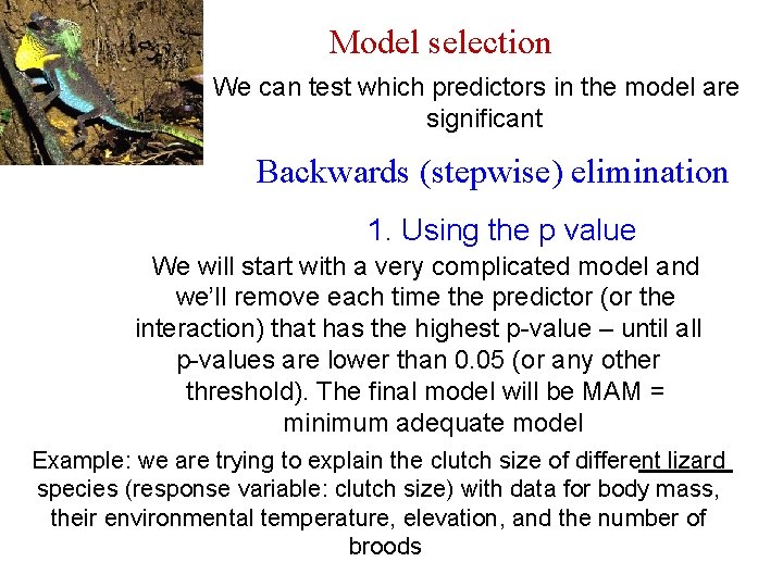
Model selection We can test which predictors in the model are significant Backwards (stepwise) elimination 1. Using the p value We will start with a very complicated model and we’ll remove each time the predictor (or the interaction) that has the highest p-value – until all p-values are lower than 0. 05 (or any other threshold). The final model will be MAM = minimum adequate model Example: we are trying to explain the clutch size of different lizard species (response variable: clutch size) with data for body mass, their environmental temperature, elevation, and the number of broods

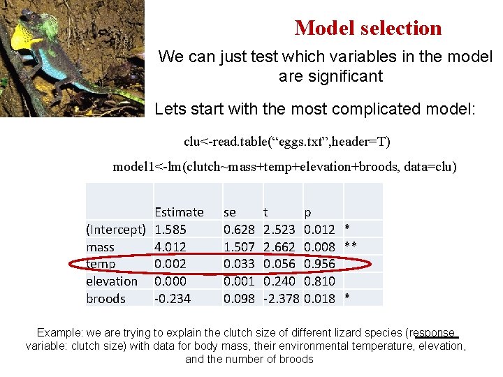
Model selection We can just test which variables in the model are significant Lets start with the most complicated model: clu<-read. table(“eggs. txt”, header=T) model 1<-lm(clutch~mass+temp+elevation+broods, data=clu) Estimate (Intercept) 1. 585 mass 4. 012 temp 0. 002 elevation 0. 000 broods -0. 234 se 0. 628 1. 507 0. 033 0. 001 0. 098 t p 2. 523 0. 012 * 2. 662 0. 008 ** 0. 056 0. 956 0. 240 0. 810 -2. 378 0. 018 * Example: we are trying to explain the clutch size of different lizard species (response variable: clutch size) with data for body mass, their environmental temperature, elevation, and the number of broods

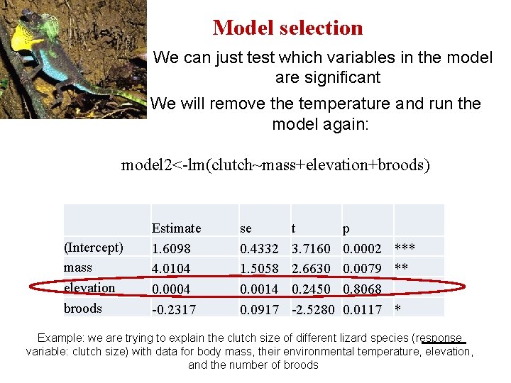
Model selection We can just test which variables in the model are significant We will remove the temperature and run the model again: model 2<-lm(clutch~mass+elevation+broods) (Intercept) mass elevation broods Estimate 1. 6098 4. 0104 0. 0004 -0. 2317 se 0. 4332 1. 5058 0. 0014 0. 0917 t 3. 7160 2. 6630 0. 2450 -2. 5280 p 0. 0002 *** 0. 0079 ** 0. 8068 0. 0117 * Example: we are trying to explain the clutch size of different lizard species (response variable: clutch size) with data for body mass, their environmental temperature, elevation, and the number of broods

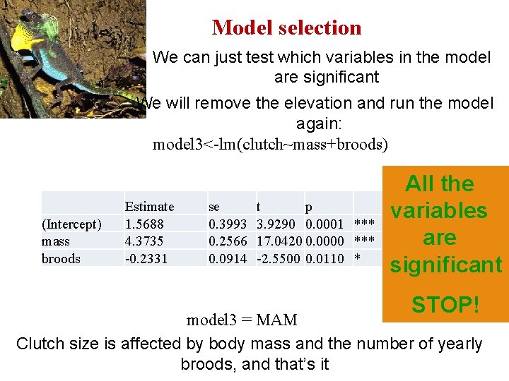
Model selection We can just test which variables in the model are significant We will remove the elevation and run the model again: model 3<-lm(clutch~mass+broods) (Intercept) mass broods Estimate 1. 5688 4. 3735 -0. 2331 se 0. 3993 0. 2566 0. 0914 t p 3. 9290 0. 0001 *** 17. 0420 0. 0000 *** -2. 5500 0. 0110 * All the variables are significant STOP! model 3 = MAM Clutch size is affected by body mass and the number of yearly broods, and that’s it

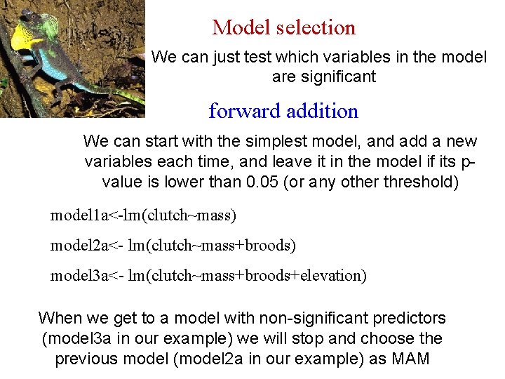
Model selection We can just test which variables in the model are significant forward addition We can start with the simplest model, and add a new variables each time, and leave it in the model if its pvalue is lower than 0. 05 (or any other threshold) model 1 a<-lm(clutch~mass) model 2 a<- lm(clutch~mass+broods) model 3 a<- lm(clutch~mass+broods+elevation) When we get to a model with non-significant predictors (model 3 a in our example) we will stop and choose the previous model (model 2 a in our example) as MAM

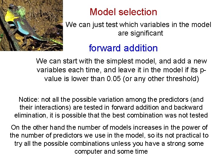
Model selection We can just test which variables in the model are significant forward addition We can start with the simplest model, and add a new variables each time, and leave it in the model if its pvalue is lower than 0. 05 (or any other threshold) Notice: not all the possible variation among the predictors (and their interactions) are tested in forward addition and backward elimination, it is possible that the best combination was not tested On the other hand the number of models increases in the power of the number of predictors we use in the model, so its not practical to try all the possible combinations unless you have a strong some computer and some time

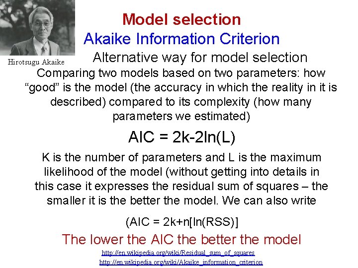
Model selection Akaike Information Criterion Hirotsugu Akaike Alternative way for model selection Comparing two models based on two parameters: how “good” is the model (the accuracy in which the reality in it is described) compared to its complexity (how many parameters we estimated) AIC = 2 k-2 ln(L) K is the number of parameters and L is the maximum likelihood of the model (without getting into details in this case it expresses the residual sum of squares – the smaller it is the better the model. We can also write (AIC = 2 k+n[ln(RSS)] The lower the AIC the better the model http: //en. wikipedia. org/wiki/Residual_sum_of_squares http: //en. wikipedia. org/wiki/Akaike_information_criterion

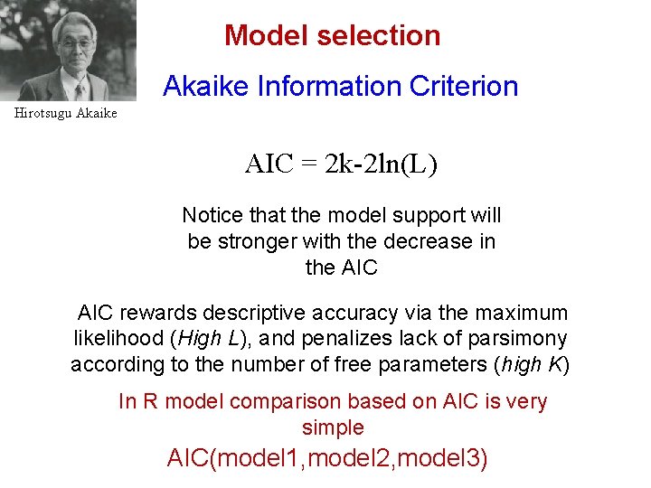
Model selection Akaike Information Criterion Hirotsugu Akaike AIC = 2 k-2 ln(L) Notice that the model support will be stronger with the decrease in the AIC rewards descriptive accuracy via the maximum likelihood (High L), and penalizes lack of parsimony according to the number of free parameters (high K) In R model comparison based on AIC is very simple AIC(model 1, model 2, model 3)

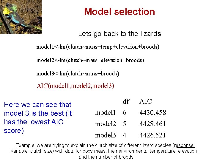
Model selection Lets go back to the lizards model 1<-lm(clutch~mass+temp+elevation+broods) model 2<-lm(clutch~mass+elevation+broods) model 3<-lm(clutch~mass+broods) AIC(model 1, model 2, model 3) Here we can see that model 3 is the best (it has the lowest AIC score) df AIC model 1 6 4430. 458 model 2 5 4428. 461 model 3 4 4426. 521 Example: we are trying to explain the clutch size of different lizard species (response variable: clutch size) with data for body mass, their environmental temperature, elevation, and the number of broods

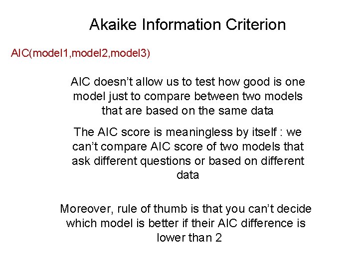
Akaike Information Criterion AIC(model 1, model 2, model 3) AIC doesn’t allow us to test how good is one model just to compare between two models that are based on the same data The AIC score is meaningless by itself : we can’t compare AIC score of two models that ask different questions or based on different data Moreover, rule of thumb is that you can’t decide which model is better if their AIC difference is lower than 2

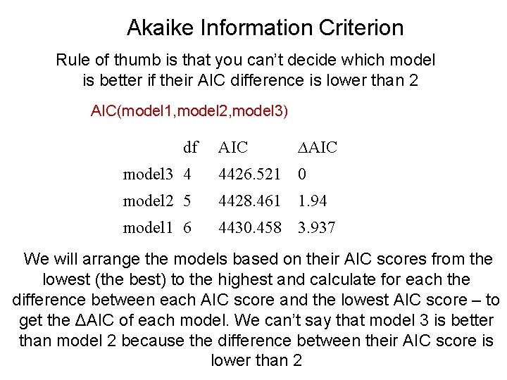
Akaike Information Criterion Rule of thumb is that you can’t decide which model is better if their AIC difference is lower than 2 AIC(model 1, model 2, model 3) df AIC ∆AIC model 3 4 4426. 521 0 model 2 5 4428. 461 1. 94 model 1 6 4430. 458 3. 937 We will arrange the models based on their AIC scores from the lowest (the best) to the highest and calculate for each the difference between each AIC score and the lowest AIC score – to get the ΔAIC of each model. We can’t say that model 3 is better than model 2 because the difference between their AIC score is lower than 2

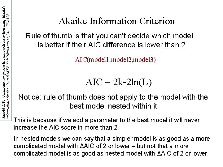
Arnold 2010. Uninformative parameters and model selection using Akaike's information criterion. Journal of Wildlife Management, 74: 1175 -1178. Akaike Information Criterion Rule of thumb is that you can’t decide which model is better if their AIC difference is lower than 2 AIC(model 1, model 2, model 3) AIC = 2 k-2 ln(L) Notice: rule of thumb does not apply to the model with the best model nested within it This is because if we add a parameter to the best model it will never increase the AIC score in more than 2 In nested models we can say that a simpler model is as good as a more complicated model with ΔAIC of 2 or lower – but not that a more complicated model is as good as nested model with ΔAIC of 2 or lower

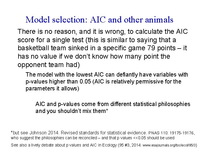
Model selection: AIC and other animals There is no reason, and it is wrong, to calculate the AIC score for a single test (this is similar to saying that a basketball team sinked in a specific game 79 points – it has no value if we don’t know how many point the opponent team had) The model with the lowest AIC can defiantly have variables with p-values higher than 0. 05 (AIC is relatively permissive for the parameters it allows) AIC and p-values come from different statistical philosophies and you shouldn’t mix them* *but see Johnson 2014. Revised standards for statistical evidence. PNAS 110: 19175 -19176, who suggest the philosophies can be reconciled – and that p values <<0. 05 should be used See also a lively debate about p values and AIC in Ecology (95 #3, 2014: www. esajournals. org/toc/ecol/95/3)

Model selection: variation on the AIC theme 1. AICc = AIC+(2 k*[k+1]/[n-k-1]) Correction to AIC for models with small sample size (http: //cran. r-project. org/web/packages/AICcmodavg. pdf R )חבילת . 2 AIC weights “Akaike weights are used in model averaging. They represent the relative likelihood of a model. To calculate them, for each model first calculate the relative likelihood of the model, which is just exp(-0. 5 * ∆AIC score for that model). The Akaike weight for a model is this value divided by the sum of these values across all models. ” † Baysian Information Criterion, BIC. 3 Less permissive 1 than AIC to large number of parameters†† 1. Notice : k is multiplied by sample size! In the AIC sample size is not incorporated BIC: -2*ln L + k*ln(n) † http: //www. brianomeara. info/tutorials/aic Aho et al. 2014. Model selection for ecologists: the worldviews of AIC and BIC. Ecology, 95: 631 -636. †† Wagenmakers & Farrell 2004

Remember for each research: "No statistical procedure can substitute for serious thinking about alternative evolutionary scenarios and their credibility" Westoby, Leishman & Lord 1995. On misinterpreting 'phylogenetic correction. J. of Ecology 83: 531 -534.