1 Wilcoxon Rank Sum Test 1 Wilcoxon with

1 Wilcoxon Rank Sum Test 1. Wilcoxon with both n 1 and n 2 < 10 2. Wilcoxon with both n 1 and n 2 ≥ 10 3. Examples Wilcoxon

2 Wilcoxon Rank Sum Test Recall from last week: § When we test a hypothesis about the difference between two independent population means, we do so using the difference between two sample means. § When the two sample variances are tested and found not to be equal § we cannot pool the sample variances § thus we cannot use the t-test for independent samples. Instead, we use the Wilcoxon Rank Sum Test. Wilcoxon

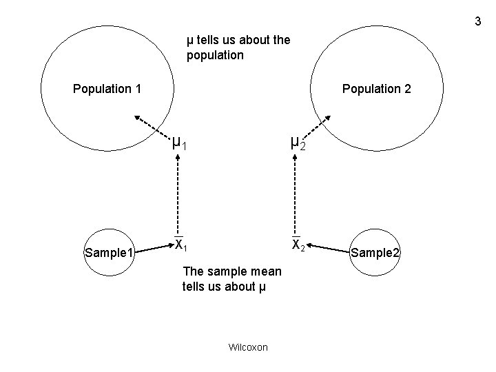
3 µ tells us about the population Population 1 Sample 1 Population 2 µ 1 µ 2 X 1 X 2 The sample mean tells us about µ Wilcoxon Sample 2

4 Wilcoxon Rank Sum Test The Z test and the t test are “parametric tests” – that is, they answer a question about the difference between populations by comparing sample statistics (e. g. , X 1 and X 2) and making an inference to the population parameters (μ 1 and μ 2). The Wilcoxon, in contrast, allows inferences about whole populations Wilcoxon

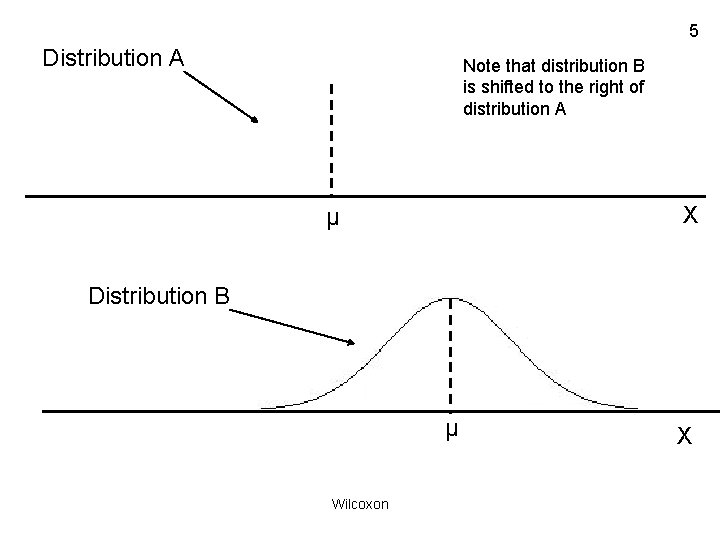
5 Distribution A Note that distribution B is shifted to the right of distribution A X μ Distribution B μ Wilcoxon X

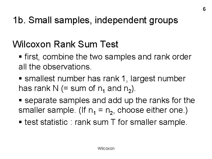
6 1 b. Small samples, independent groups Wilcoxon Rank Sum Test § first, combine the two samples and rank order all the observations. § smallest number has rank 1, largest number has rank N (= sum of n 1 and n 2). § separate samples and add up the ranks for the smaller sample. (If n 1 = n 2, choose either one. ) § test statistic : rank sum T for smaller sample. Wilcoxon

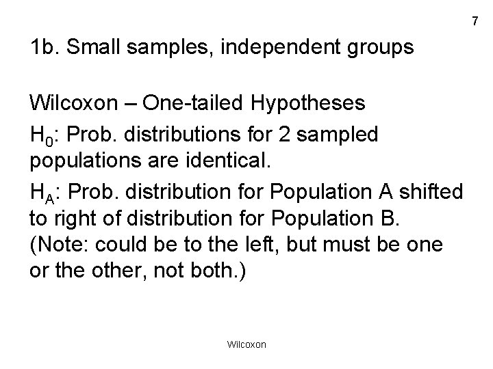
7 1 b. Small samples, independent groups Wilcoxon – One-tailed Hypotheses H 0: Prob. distributions for 2 sampled populations are identical. HA: Prob. distribution for Population A shifted to right of distribution for Population B. (Note: could be to the left, but must be one or the other, not both. ) Wilcoxon

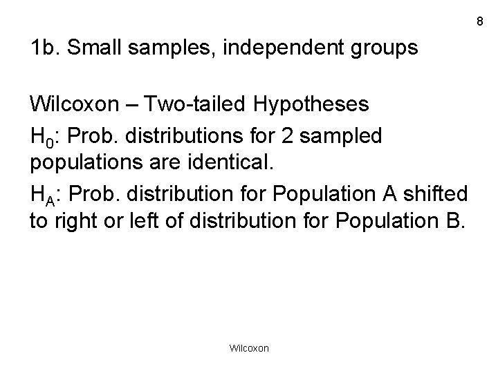
8 1 b. Small samples, independent groups Wilcoxon – Two-tailed Hypotheses H 0: Prob. distributions for 2 sampled populations are identical. HA: Prob. distribution for Population A shifted to right or left of distribution for Population B. Wilcoxon

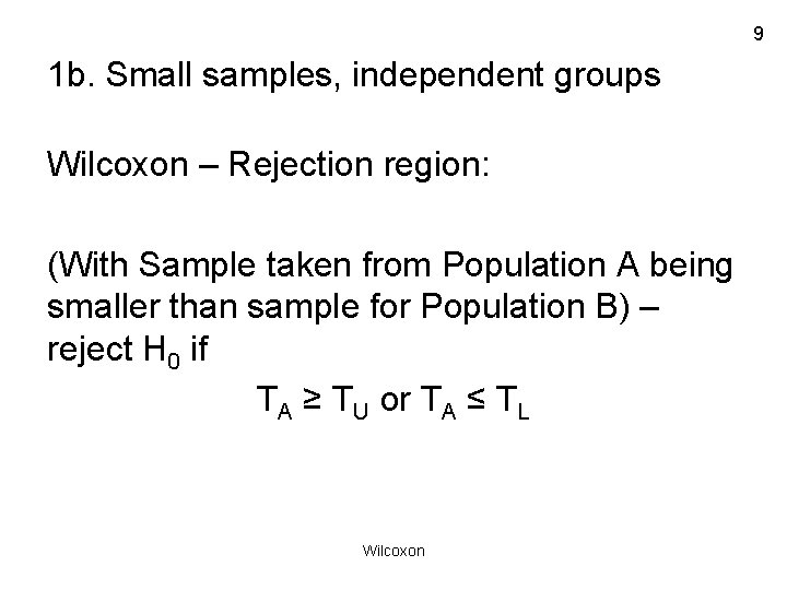
9 1 b. Small samples, independent groups Wilcoxon – Rejection region: (With Sample taken from Population A being smaller than sample for Population B) – reject H 0 if TA ≥ TU or TA ≤ TL Wilcoxon

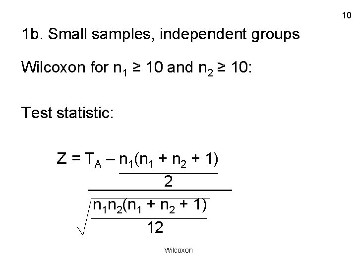
10 1 b. Small samples, independent groups Wilcoxon for n 1 ≥ 10 and n 2 ≥ 10: Test statistic: Z = TA – n 1(n 1 + n 2 + 1) 2 n 1 n 2(n 1 + n 2 + 1) 12 Wilcoxon

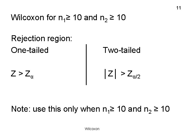
11 Wilcoxon for n 1≥ 10 and n 2 ≥ 10 Rejection region: One-tailed Two-tailed Z > Zα │Z│ > Zα/2 Note: use this only when n 1≥ 10 and n 2 ≥ 10 Wilcoxon

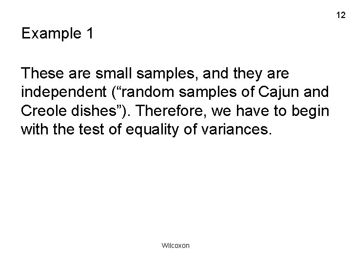
12 Example 1 These are small samples, and they are independent (“random samples of Cajun and Creole dishes”). Therefore, we have to begin with the test of equality of variances. Wilcoxon

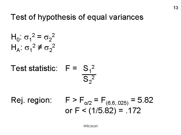
13 Test of hypothesis of equal variances H 0 : 1 2 = 2 2 H A : 1 2 ≠ 2 2 Test statistic: F = S 12 S 22 Rej. region: F > Fα/2 = F(6, 6, . 025) = 5. 82 or F < (1/5. 82) =. 172 Wilcoxon

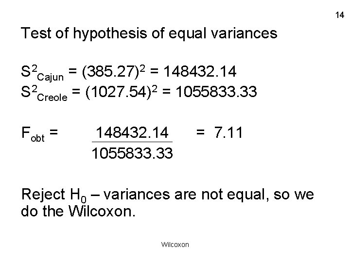
14 Test of hypothesis of equal variances S 2 Cajun = (385. 27)2 = 148432. 14 S 2 Creole = (1027. 54)2 = 1055833. 33 Fobt = 148432. 14 1055833. 33 = 7. 11 Reject H 0 – variances are not equal, so we do the Wilcoxon

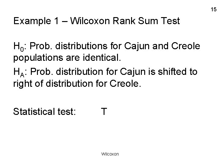
15 Example 1 – Wilcoxon Rank Sum Test H 0: Prob. distributions for Cajun and Creole populations are identical. HA: Prob. distribution for Cajun is shifted to right of distribution for Creole. Statistical test: T Wilcoxon

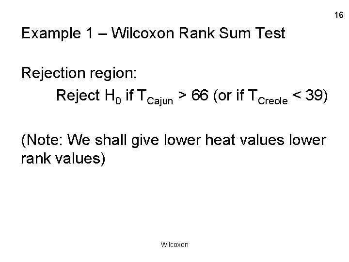
16 Example 1 – Wilcoxon Rank Sum Test Rejection region: Reject H 0 if TCajun > 66 (or if TCreole < 39) (Note: We shall give lower heat values lower rank values) Wilcoxon

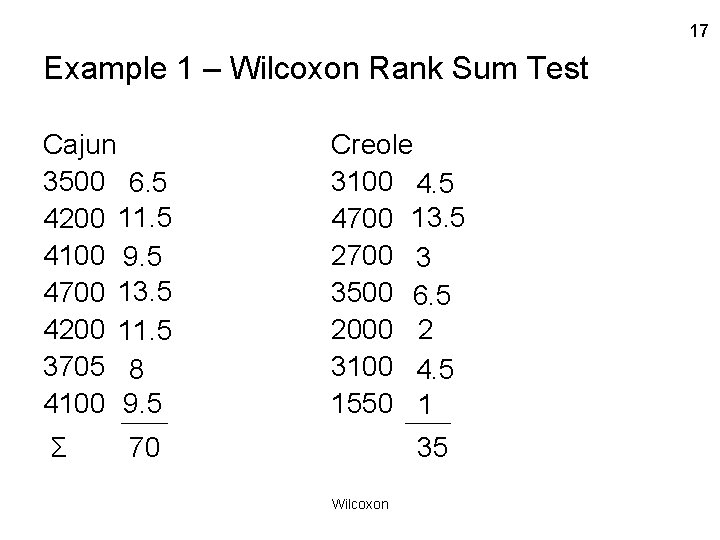
17 Example 1 – Wilcoxon Rank Sum Test Cajun 3500 6. 5 4200 11. 5 4100 9. 5 4700 13. 5 4200 11. 5 3705 8 4100 9. 5 Σ Creole 3100 4. 5 4700 13. 5 2700 3 3500 6. 5 2000 2 3100 4. 5 1550 1 70 35 Wilcoxon

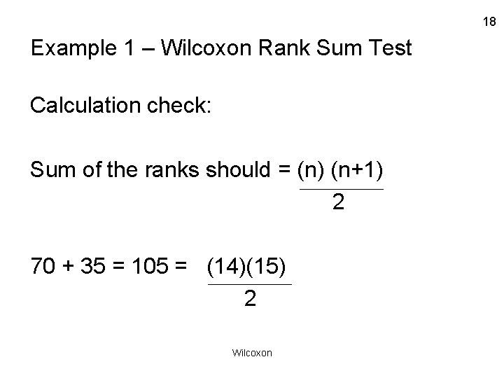
18 Example 1 – Wilcoxon Rank Sum Test Calculation check: Sum of the ranks should = (n) (n+1) 2 70 + 35 = 105 = (14)(15) 2 Wilcoxon

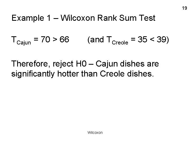
19 Example 1 – Wilcoxon Rank Sum Test TCajun = 70 > 66 (and TCreole = 35 < 39) Therefore, reject H 0 – Cajun dishes are significantly hotter than Creole dishes. Wilcoxon

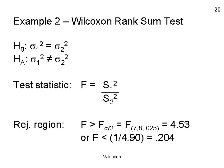
20 Example 2 – Wilcoxon Rank Sum Test H 0 : 1 2 = 2 2 H A : 1 2 ≠ 2 2 Test statistic: F = S 12 S 22 Rej. region: F > Fα/2 = F(7, 8, . 025) = 4. 53 or F < (1/4. 90) =. 204 Wilcoxon

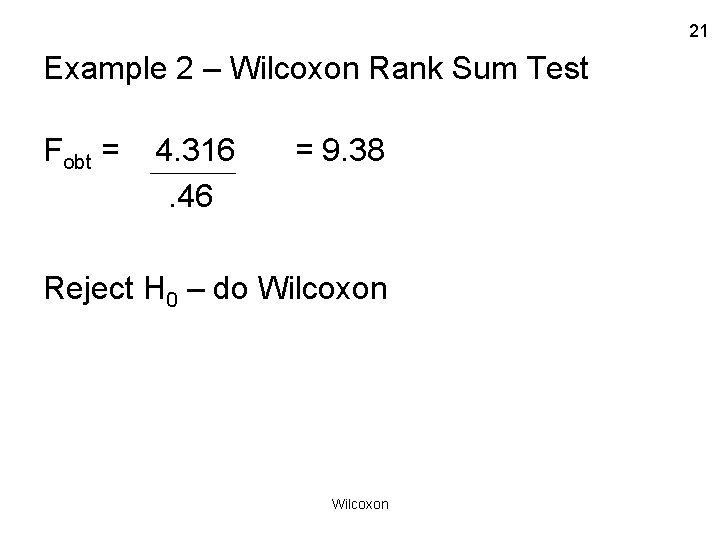
21 Example 2 – Wilcoxon Rank Sum Test Fobt = 4. 316. 46 = 9. 38 Reject H 0 – do Wilcoxon

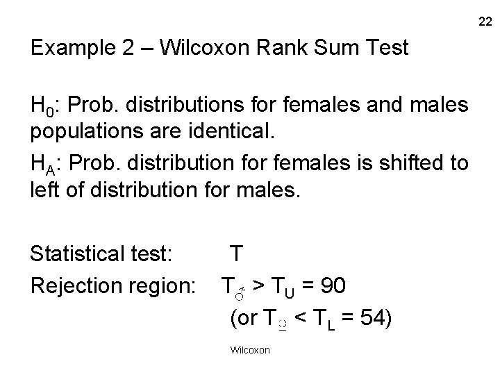
22 Example 2 – Wilcoxon Rank Sum Test H 0: Prob. distributions for females and males populations are identical. HA: Prob. distribution for females is shifted to left of distribution for males. Statistical test: Rejection region: T T♂ > TU = 90 (or T♀ < TL = 54) Wilcoxon

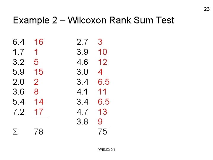
23 Example 2 – Wilcoxon Rank Sum Test 6. 4 1. 7 3. 2 5. 9 2. 0 3. 6 5. 4 7. 2 16 1 5 15 2 8 14 17 Σ 78 2. 7 3. 9 4. 6 3. 0 3. 4 4. 1 3. 4 4. 7 3. 8 3 10 12 4 6. 5 11 6. 5 13 9 75 Wilcoxon

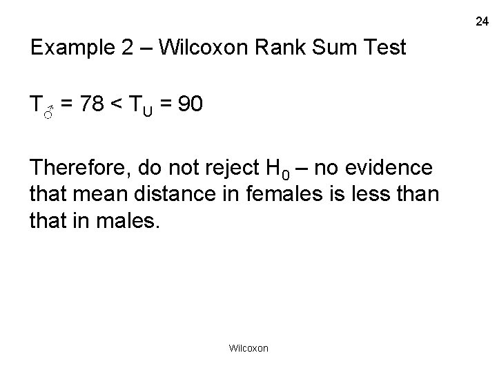
24 Example 2 – Wilcoxon Rank Sum Test T♂ = 78 < TU = 90 Therefore, do not reject H 0 – no evidence that mean distance in females is less than that in males. Wilcoxon

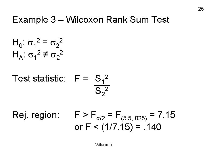
25 Example 3 – Wilcoxon Rank Sum Test H 0 : 1 2 = 2 2 H A : 1 2 ≠ 2 2 Test statistic: F = S 12 S 22 Rej. region: F > Fα/2 = F(5, 5, . 025) = 7. 15 or F < (1/7. 15) =. 140 Wilcoxon

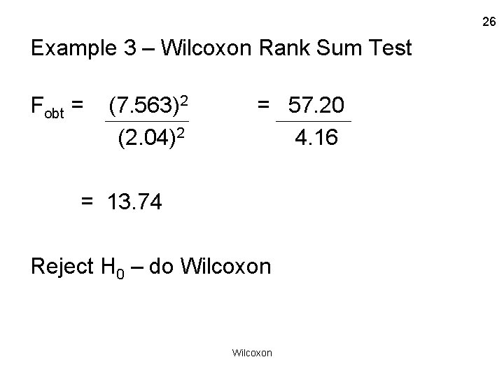
26 Example 3 – Wilcoxon Rank Sum Test Fobt = (7. 563)2 (2. 04)2 = 57. 20 4. 16 = 13. 74 Reject H 0 – do Wilcoxon

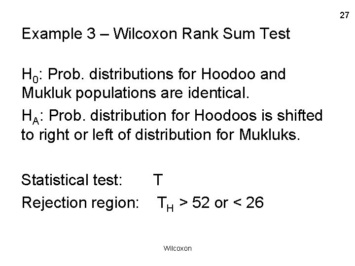
27 Example 3 – Wilcoxon Rank Sum Test H 0: Prob. distributions for Hoodoo and Mukluk populations are identical. HA: Prob. distribution for Hoodoos is shifted to right or left of distribution for Mukluks. Statistical test: T Rejection region: TH > 52 or < 26 Wilcoxon

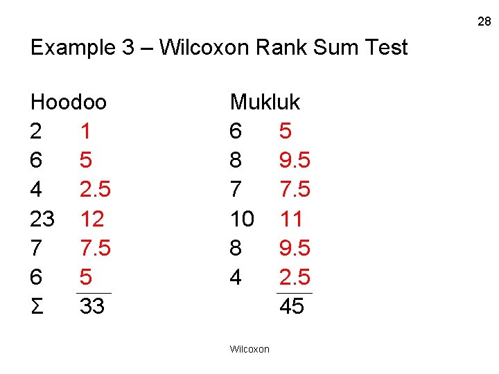
28 Example 3 – Wilcoxon Rank Sum Test Hoodoo 2 1 6 5 4 2. 5 23 12 7 7. 5 6 5 Σ 33 Mukluk 6 5 8 9. 5 7 7. 5 10 11 8 9. 5 4 2. 5 45 Wilcoxon

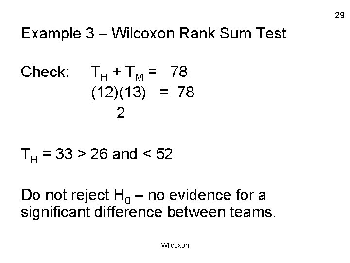
29 Example 3 – Wilcoxon Rank Sum Test Check: TH + TM = 78 (12)(13) = 78 2 TH = 33 > 26 and < 52 Do not reject H 0 – no evidence for a significant difference between teams. Wilcoxon