NJ CLEAN AIR COUNCIL Fine Particulate Matter in

NJ CLEAN AIR COUNCIL Fine Particulate Matter in the Atmosphere April 14, 2004 Topic: Health Effects of Ambient Air Pollution: The Influence of Particle Properties and Composition Presented by: Morton Lippmann, Ph. D. Professor of Environmental Medicine NYU School of Medicine Tuxedo, NY 10987 Acknowledgements: Research supported by Center Grants from EPA (R 827351) and NIEHS (ES 00260).

INTRODUCTION • Primary (Health Protective) National Ambient Air Quality Standards (NAAQS) have been established on the basis of demonstrated associations between ambient air concentrations and health-related measures in human population groups.

• NAAQS have been established for: Photochemical Oxidants, currently indexed by ozone (O 3) for 8 hr daily max. Nitrogen Oxides (NOx), indexed by nitrogen dioxide (NO 2) for annual av. Sulfur Oxides (SOx), indexed by sulfur dioxide (SO 2) for 24 hr daily max. and annual av. Lead (Pb, all forms) - for 3 month av. Particulate Matter (PM), for 24 hr daily max. and annual av. currently indexed by: PM 2. 5 (50% cut at 2. 5 µm aerodynamic diameter) PM 10 (50% cut at 10 µm aerodynamic diameter), which may be replaced by PM 10 -2. 5 in 2004 or 2005

• Health Effects Basis for NAAQS (Major Influence): Premature Mortality (PM, and possibly for SOx) Hospital Admissions (O 3, PM) Angina (CO) Immune System Dysfunction (NO 2) Neurobehavioral Deficits (Pb) Increased Blood Pressure (Pb) • Widespread NAAQS Exceedances for: O 3 PM 2. 5

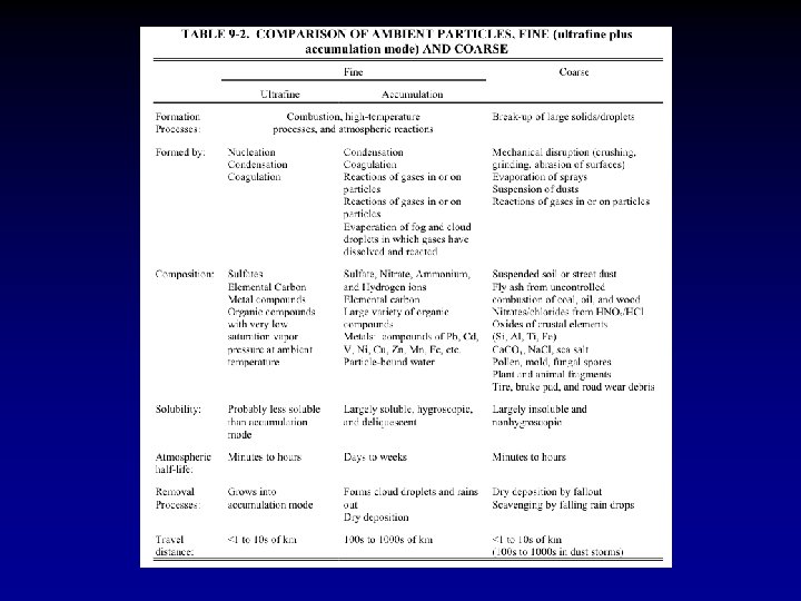
Figure 9 -6. An idealized distribution of ambient particulate matter showing the accumulation mode and the coarse mode and the size fractions collected by size-selective samplers. (WRAC is the Wide Range Aerosol Classifier which collects the entire coarse model [Lundgren and Burton, 1995]). Source: 4 th Draft PM Criteria Document, June 2003.

Figure 9 -4. Submicron number size distributions observed in a boreal forest in Finland showing the tri-modal structure of fine particles. The total particle number concentration was 1011 particles/cm 3 (10 minute average). Source: 4 th Draft PM Criteria Document, June 2003.

Figure 9 -7. Schematic showing major nonvolatile and semivolatile components of PM 2. 5. Semivolatile components are subject to partial to complete loss during equilibration or heating. The optimal technique would be to remove all particle-bound water but no ammonium nitrate or semivolatile organic PM. Source: 4 th Draft PM Criteria Document, June 2003.

Figure 9 -8. Major chemical components of PM 2. 5 as determined in the U. S. Environmental Protection Agency’s national speciation network from October 2001 to September 2002. Source: 4 th Draft PM Criteria Document, June 2003.

Figure 9 -10. Regression analysis of daytime total personal exposures to PM 10 versus ambient PM 10 concentrations using data from the PTEAM study. The slope of the regression line is interpreted by exposure analysts as the average , where C = A. Source: 4 th Draft PM Criteria Document, June 2003.

Figure 9 -11. Regression analysis daytime exposures to the ambient component of personal exposure to PM 10 (ambient exposure) versus ambient PM 10 concentrations. Source: 4 th Draft PM Criteria Document, June 2003.

Figure 2 -8. Average measured annual mean PM 2. 5 concentration trend at IMPROVE sites, 19922001. Included sites must have 8 of 10 valid years of data; missing years are interpolated. Measured mass represents measurement from the filter. Source: 1 st Draft PM Staff Paper, August 2003.

Figure 2 -4. Distribution of annual mean PM 2. 5 and estimated annual mean PM 10 -2. 5 concentrations by region, 2000 -2002. Box depicts interquartile range and median; whiskers depict 5 th and 95 th percentiles; asterisks depict minimum and maximum. Number below indicates the number of sites in each region. Source: 1 st Draft PM Staff Paper, August 2003.

Figure 6 -12. Diagram of known and suspected clearance pathways for poorly soluble particles depositing in the alveolar region. (The magnitude of various pathways may depend upon size of deposited particle. ) Source: 4 th Draft PM Criteria Document, June 2003.

Figure 9 -1. A general framework for integrating particulate-matter research. Note that this figure is not intended to represent a framework for research management. Such a framework would include multiple pathways for the flow of information. Source: 4 th Draft PM Criteria Document, June 2003.

Figure 8 -9. Natural logarithm of relative risk for total and cause-specific mortality per 10 µg/m 3 PM 2. 5 (approximately the excess relative risk as a fraction), with smoothed concentrationresponse functions. Based on Pope et al. (2002) mean curve (solid line) with pointwise 95% confidence intervals (dashed lines).

Figure 8 -11. Relative risk of total and cause-specific mortality for particle metrics and gaseous pollutants over different averaging periods (years 1979 -2000 in parentheses). Source: 4 th Draft PM Criteria Document, June 2003.

Figure 4 -8. Estimated annual percent of mortality associated with long-term exposure to PM 2. 5 (and 95% confidence interval): Single-pollutant and multi-pollutant models. (Single-pollutant models are always on the left, followed by the corresponding multi-pollutant models. ) Source: 1 st Draft PM Staff Paper, August 2003.

Figure 3 -5. Effect estimates for PM 2. 5 and mortality from total, respiratory and cardiovascular causes from U. S. and Canadian cities in relation to the mortality-days product (the product of study days and the number of deaths per day - an indicator of study precision). Study locations are identified below; multi-city studies denoted by a star. Results of GAM stringent reanalyses; studies not originally using GAM denoted by • . Source: 1 st Draft PM Staff Paper, August 2003.

Figure 3 -12. Associations between PM 2. 5 and total mortality from U. S. studies, plotted against gaseous pollutant concentrations from the same locations. Air quality data obtained from the Aerometric Information Retrieval System (AIRS) for each study time period: (A) mean of 4 th highest 8 -hour ozone concentration; (B) mean of 2 nd highest 1 -hour NO 2 concentration; (C) mean of 2 nd highest 24 -hour SO 2 concentration; (D) mean of 2 nd highest 8 -hour CO concentration; (E) annual mean SO 2 concentration; (F) annual mean NO 2 concentration. Study locations are identified below. Source: 1 st Draft PM Staff Paper, August 2003.

Figure 3 -11 a. Estimated excess mortality and morbidity risks per 25 µg/m 3 PM 2. 5 from U. S. and Canadian studies (above). Results of GAM stringent reanalyses; studies not originally using GAM denoted by • . Multi-city studies denoted by a star. Source: 1 st Draft PM Staff Paper, August 2003.

Figure 3 -11 b. Estimated excess mortality and morbidity risks per 25 µg/m 3 PM 10 -2. 5 from U. S. and Canadian studies (above). Results of GAM stringent reanalyses; studies not originally using GAM denoted by • . Multi-city studies denoted by a star. Source: 1 st Draft PM Staff Paper, August 2003.

Figure 8 -19. Marginal posterior distribution for effects of PM 10 on all cause mortality at lag 0, 1, and 2 for the 90 cities. From Dominici et al. (2002 a). The numbers in the upper right legend are posterior probabilities that overall effects are greater than 0. Source: 4 th Draft PM Criteria Document, June 2003.

Figure 8 -6. Marginal posterior distributions for effect of PM 10 on total mortality at lag 1 with and without control for other pollutants, for the 90 cities. The numbers in the upper right legend are the posterior probabilities that the overall effects are greater than 0. Source: 4 th Draft PM Criteria Document, June 2003.

From: Zanobetti, et al. , Environ. Health Perspect. 111: 1188 -1193 (2003).

Source: 1 st Draft PM Staff Paper, August 2003.

Figure 8 -13. Percent change in hospital admission rates and 95% CIs for an IQR increase in pollutants from singlepollutant models for asthma. Poisson regression models are adjusted for time trends (64 -df spline), day-of-week, and temperature (4 -df spline). The IQR for each pollutant equals: 19 µg/m 3 for PM 10, 11. 8 µg/m 3 for PM 2. 5, 9. 3 µg/m 3 for coarse PM, 20 ppb for O 3, 4. 9 ppb for SO 2, and 924 ppb for CO. Triplets of estimates for each pollutant are for the original GAM analysis using smoothing splines, the revised GAM analysis with stricter convergence criteria, and the GLM analysis with natural splines. For pollutants that required imputation (i. e. , estimation of missing value) estimates ignoring (single imputation) or adjusting for (multiple imputation) the imputation are shown. Source: 4 th Draft PM Criteria Document, June 2003.

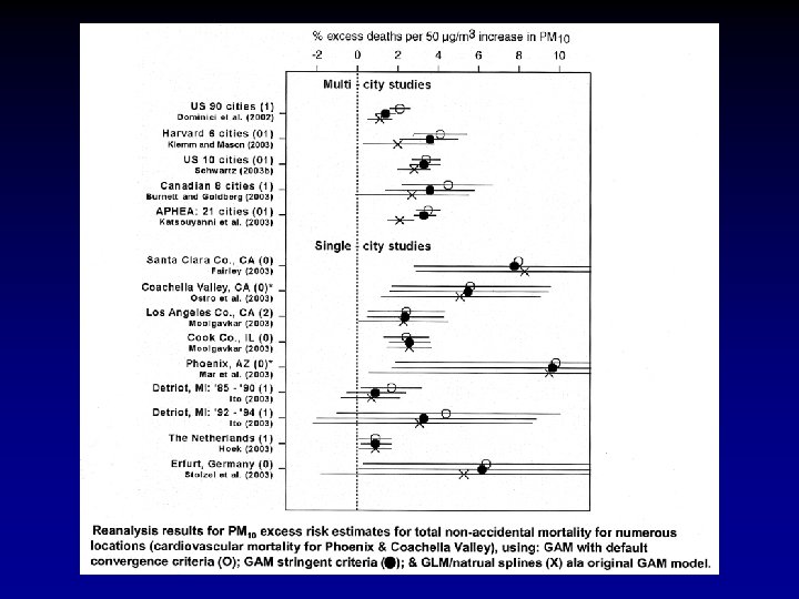
Figure 8 -14. Maximum excess risk of respiratory-related hospital admissions and visits per 50 µg/m 3 PM 10 increment in selected studies of U. S. cities based on single-pollutant models.

Figure 9 -18. Acute cardiovascular hospitalizations and PM exposure excess risk estimates derived from selected U. S. PM 10 studies. CVD = cardiovascular disease and CHF = congestive heart failure. IHD = ischemic heart disease.

Unresolved Problems in Characterizing Health Effects of Ambient Air Pollution • • • lack of demonstrated biological mechanisms for PM-related effects, potential influence of measurement error and exposure error, potential confounding by copollutants, evaluation of the effects of components, surface coatings or other characteristics of PM, the shape of concentration-response relationships, methodological uncertainties in epidemiological analyses, the extent of life span shortening, characterization of annual and daily background concentrations, understanding of the effects of coarse fraction PM, and effects, if any, of air toxics.

1. 8 1. 6 Boys Unidirectional case-crossover Bidirectional case-crossover Time-series Relative Risk Estimates 1. 4 1. 2 1. 0 0. 8 1. 6 Girls 1. 4 1. 2 1. 0 0. 8 1 -day 2 -day 3 -day 4 -day 5 -day Exposure Averaging 6 -day 7 -day Asthma hospital admission RR estimates and 95% Cls for PM 10 -2. 5 for children 6 -12 years old, Toronto, 1981 -1993, adjusted for weather conditions, using case-crossover and time-series analysis. From: Lin et al. , Environ. Health Perspect, 110: 575 -581, 2002

50 LUNG A HEART B * CAPS Filtered Air CL (cps/cm 2) 40 50 ** 50 40 40 30 30 30 20 20 10 10 10 0 0 1 2 3 4 5 LIVER C 20 0 1 2 3 4 Time (hr) 5 0 1 2 3 4 5 Time course of increase of in situ chemiluminescence (CL) from lung (A), heart (B), and liver (C) of rats exposed to CAPs (average mass concentration, 300 ± 60 mg/m 3) or filtered air for 1, 3, and 5 hr. Each point represents the mean ± SEM (n=10 determinations). Compared with sham controls or with time 0, *p<0. 001 and **p<0. 005. From: Gurgueira et al. , Environmental Health Perspectives, v 10: 749 -755, Aug. 2002