Network Modeling for Psychological and Attitudinal Data 11012017

Network Modeling for Psychological (and Attitudinal) Data 11/01/2017 – 12/01/2017 Oldenburg Adela Isvoranu & Pia Tio http: //www. adelaisvoranu. com/Oldenburg 2018

Workshop Overview • Thursday January 11 • Morning • • Introduction & Theoretical Foundation of Network Analysis Drawing Networks in R (part of practical) Afternoon • Network Estimation(Markov Random Fields: Gaussian Graphical Model & Ising Model) • Estimating Networks in R Friday January 12 • Morning • • Network Stability Afternoon • Advanced Methods (Network Comparison Test, Mixed Graphical Models, Latent Variable Network Modeling)

Afternoon Session Overview Advanced methods • Part 1. Network Comparison Test • Part 2. Mixed Graphical Models • Part 3. Latent Variable Network Modeling Practical Session Any questions you have

Afternoon Session Overview Advanced methods • Part 1. Network Comparison Test • Part 2. Mixed Graphical Models • Part 3. Latent Variable Network Modeling Practical Session Any questions you have

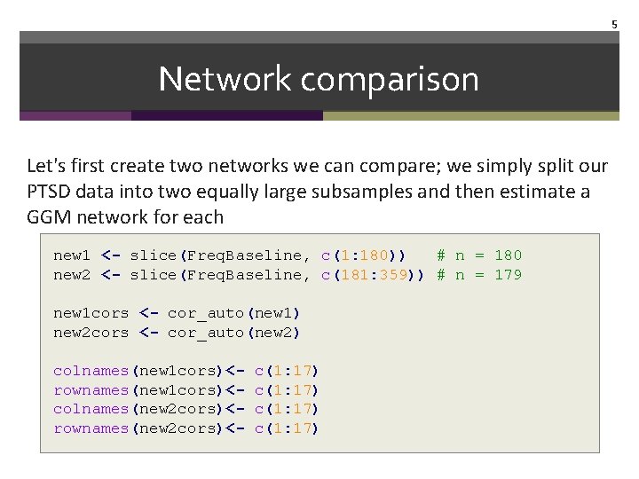
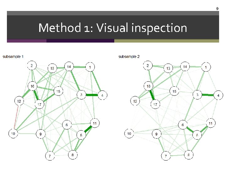
5 Network comparison Let's first create two networks we can compare; we simply split our PTSD data into two equally large subsamples and then estimate a GGM network for each new 1 <- slice(Freq. Baseline, c(1: 180)) # n = 180 new 2 <- slice(Freq. Baseline, c(181: 359)) # n = 179 new 1 cors <- cor_auto(new 1) new 2 cors <- cor_auto(new 2) colnames(new 1 cors)<rownames(new 1 cors)<colnames(new 2 cors)<rownames(new 2 cors)<- c(1: 17)

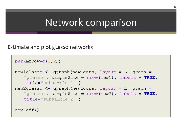
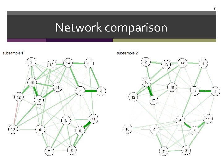
6 Network comparison Estimate and plot g. Lasso networks par(mfrow=c(1, 2)) new 1 glasso <- qgraph(new 1 cors, layout "glasso", sample. Size = nrow(new 1), title="subsample 1" ) new 2 glasso <- qgraph(new 2 cors, layout "glasso", sample. Size = nrow(new 2), title="subsample 2" ) dev. off() = L, graph = labels = TRUE,

7 Network comparison

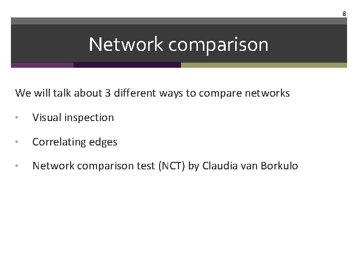
8 Network comparison We will talk about 3 different ways to compare networks • Visual inspection • Correlating edges • Network comparison test (NCT) by Claudia van Borkulo

9 Method 1: Visual inspection

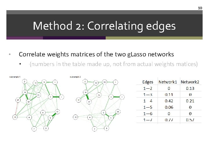
10 Method 2: Correlating edges • Correlate weights matrices of the two g. Lasso networks • (numbers in the table made up, not from actual weights matices)

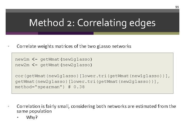
11 Method 2: Correlating edges • Correlate weights matrices of the two g. Lasso networks new 1 m <- get. Wmat(new 1 glasso) new 2 m <- get. Wmat(new 2 glasso) cor(get. Wmat(new 1 glasso)[lower. tri(get. Wmat(new 1 glasso))], get. Wmat(new 2 glasso)[lower. tri(get. Wmat(new 2 glasso))], method="spearman") # 0. 38 • Correlation is fairly small, considering both networks are estimated from the same population • Why?

12 Method 2: Correlating edges • GGM is regularized, and regularization depends on sample size: smaller N �higher uncertainty �more severe regularization. Many 0 s reduce (or increase? ) the correlation • Would we expect that the correlation among unregularized networks is larger?

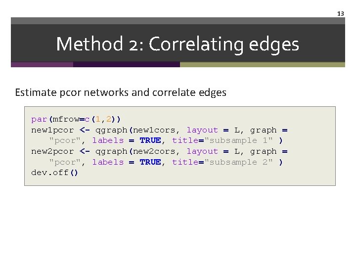
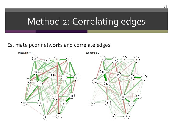
13 Method 2: Correlating edges Estimate pcor networks and correlate edges par(mfrow=c(1, 2)) new 1 pcor <- qgraph(new 1 cors, layout = L, graph = "pcor", labels = TRUE, title="subsample 1" ) new 2 pcor <- qgraph(new 2 cors, layout = L, graph = "pcor", labels = TRUE, title="subsample 2" ) dev. off()

14 Method 2: Correlating edges Estimate pcor networks and correlate edges

15 Method 2: Correlating edges Estimate pcor networks and correlate adjacency matrices: new 1 mpcor <- get. Wmat(new 1 pcor) new 2 mpcor <- get. Wmat(new 2 pcor)

16 Method 2: Correlating edges cor(get. Wmat(new 1 mpcor)[lower. tri(get. Wmat(new 1 mpcor))], get. Wmat(new 2 mpcor)[lower. tri(get. Wmat(new 2 mpcor))], method="spearman") #0. 13

17 Method 2: Correlating edges Let's look at the bootnet output of the pcor network

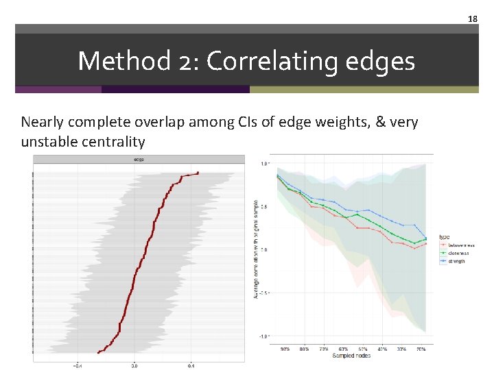
18 Method 2: Correlating edges Nearly complete overlap among CIs of edge weights, & very unstable centrality

19 Method 2: Correlating edges Main messages: • Correlating edges can be useful, but does not provide a proper test statistic • Behavior of this "test" is not well understood • Problematic especially in small N

20 Method 3: Network Comparison Tests We will talk about 3 tests here, using the R-package Network. Comparison. Test A. Global strength invariance test (independent & dependent) B. Network structure invariance test C. Edge strength invariance test Claudia van Borkulo https: //cvborkulo. com https: //github. com/cvborkulo/Network. Comparison. Test

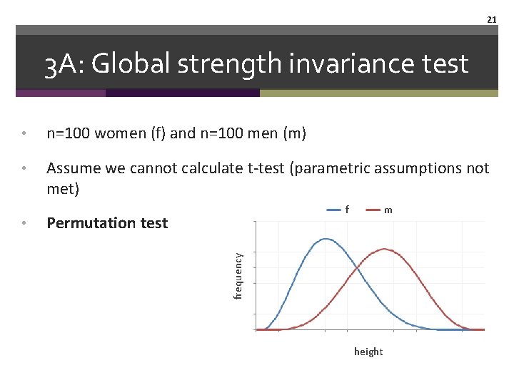
21 3 A: Global strength invariance test • n=100 women (f) and n=100 men (m) • Assume we cannot calculate t-test (parametric assumptions not met) Permutation test m frequency • f height

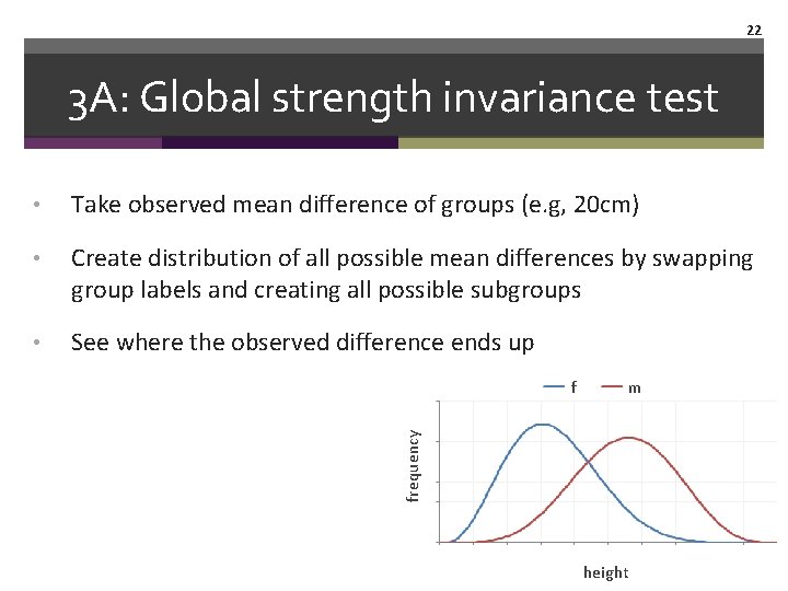
22 3 A: Global strength invariance test • Take observed mean difference of groups (e. g, 20 cm) • Create distribution of all possible mean differences by swapping group labels and creating all possible subgroups • See where the observed difference ends up m frequency f height

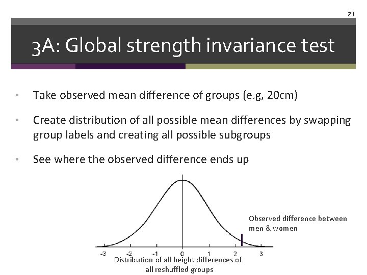
23 3 A: Global strength invariance test • Take observed mean difference of groups (e. g, 20 cm) • Create distribution of all possible mean differences by swapping group labels and creating all possible subgroups • See where the observed difference ends up Observed difference between men & women Distribution of all height differences of all reshuffled groups

24 3 A: Global strength invariance test • Global strength invariance test: permutation test of absolute sum of all edges of two networks • Observed difference between 2 networks: observed difference of absolute sum of edges (e. g. , 3. 5 points) • Permutation: shuffle individuals across the 2 groups, estimate network, obtain difference of absolute sum of edges, create distribution under H 0 • See how probable the observed difference is

25 3 A: Global strength invariance test • We compare reduced 11 -item versions of our 2 prior PTSD subsamples again (not enough power for 17 items) library(Network. Comparison. Test) new 1 x <- slice(Freq. Baseline, c(1: 180)) new 2 x <- slice(Freq. Baseline, c(181: 359)) new 1 x[, 1: 17] <- sapply(new 1[, 1: 17], as. numeric) new 2 x[, 1: 17] <- sapply(new 2[, 1: 17], as. numeric) new 1 x <- select(new 1 x, 5: 15) new 2 x <- select(new 2 x, 5: 15)

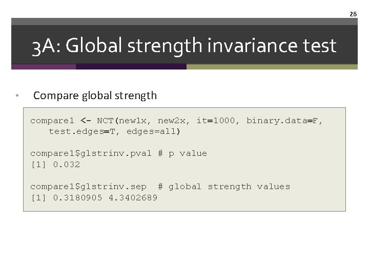
26 3 A: Global strength invariance test • Compare global strength compare 1 <- NCT(new 1 x, new 2 x, it=1000, binary. data=F, test. edges=T, edges=all) compare 1$glstrinv. pval # p value [1] 0. 032 compare 1$glstrinv. sep # global strength values [1] 0. 3180905 4. 3402689

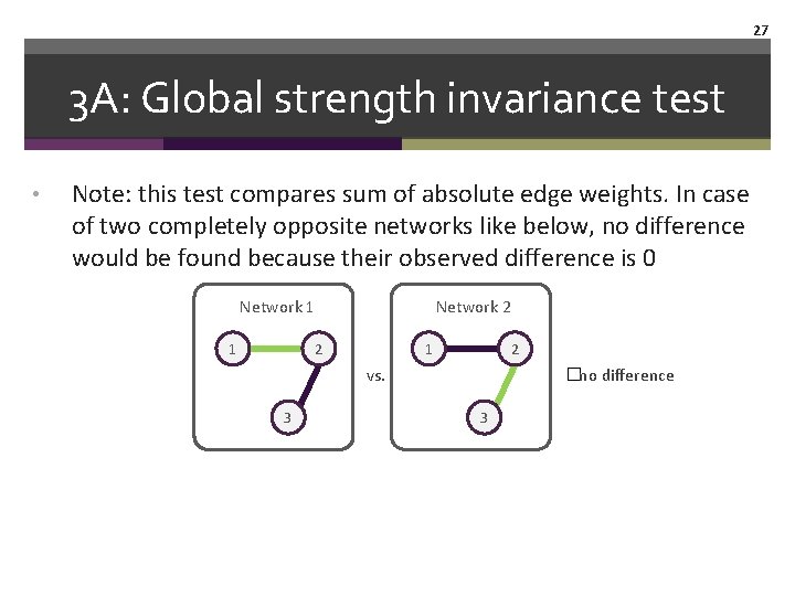
27 3 A: Global strength invariance test • Note: this test compares sum of absolute edge weights. In case of two completely opposite networks like below, no difference would be found because their observed difference is 0 Network 1 1 Network 2 2 1 2 vs. 3 �no difference 3

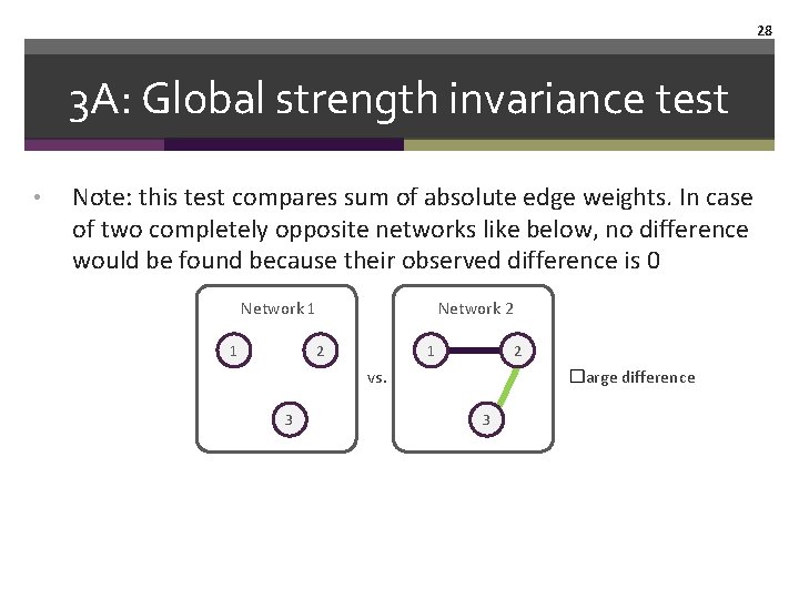
28 3 A: Global strength invariance test • Note: this test compares sum of absolute edge weights. In case of two completely opposite networks like below, no difference would be found because their observed difference is 0 Network 1 1 Network 2 2 1 2 vs. 3 �large difference 3

29 3 A: Global strength invariance test • There is also a dependent version of this test that can be used to compare two networks in the same population across time • In this case, we simply add paired = TRUE to the code of the NCT compare 1 <- NCT(new 1 x, new 2 x, paired=TRUE)

30 3 B: Network structure invariance test • This is what most of us actually want — a test that compares the structures of networks compare 1 <- NCT(new 1 x, new 2 x, it=1000, binary. data=F, test. edges=T, edges=all) compare 1$nwinv. pval# p value [1] 0. 005

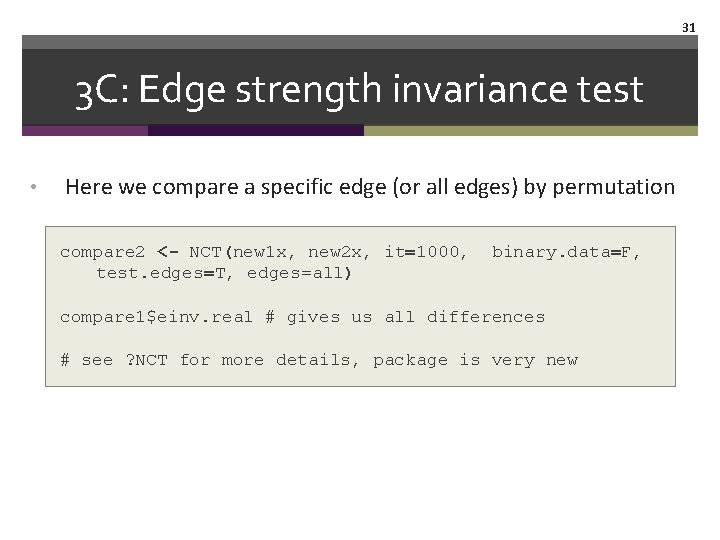
31 3 C: Edge strength invariance test • Here we compare a specific edge (or all edges) by permutation compare 2 <- NCT(new 1 x, new 2 x, it=1000, test. edges=T, edges=all) binary. data=F, compare 1$einv. real # gives us all differences # see ? NCT for more details, package is very new

Note • NCT has been tested for binary-only and continious~normalonly data • • You can manually adjust the code to be able to use it for ordinal data NCT can only compare two networks at once

Afternoon Session Overview Advanced methods • Part 1. Network Comparison Test • Part 2. Mixed Graphical Models • Part 3. Latent Variable Network Modeling Practical Session Any questions you have

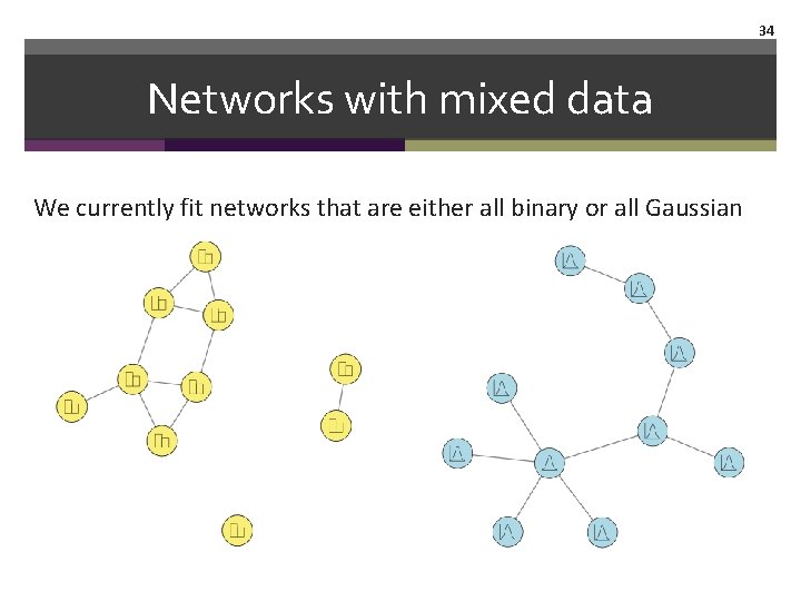
34 Networks with mixed data We currently fit networks that are either all binary or all Gaussian

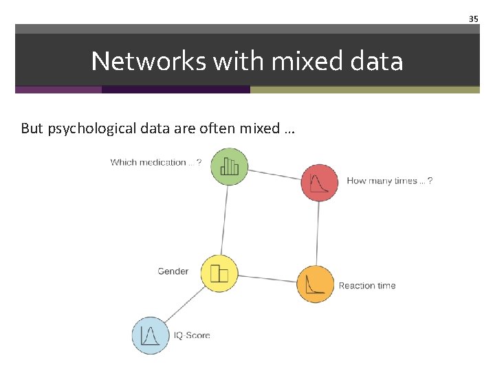
35 Networks with mixed data But psychological data are often mixed …

Networks with mixed data • It is possible to estimate networks for such data from mixed continous models, however • • information loss due to transformations cannot incorporate categorical and nominal variables

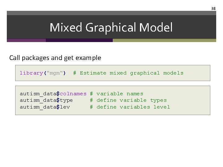
37 Mixed Graphical Model • Novel R package mgm (mixed graphical models) allows us to fix mixed data • • By Jonas Haslbeck, Uv. A, http: //jmbh. github. io/papers_software Works similar to the Ising model • Bunch of different multiple regressions

38 Mixed Graphical Model Call packages and get example library("mgm") # Estimate mixed graphical models autism_data$colnames # variable names autism_data$type # define variable types autism_data$lev # define variables level

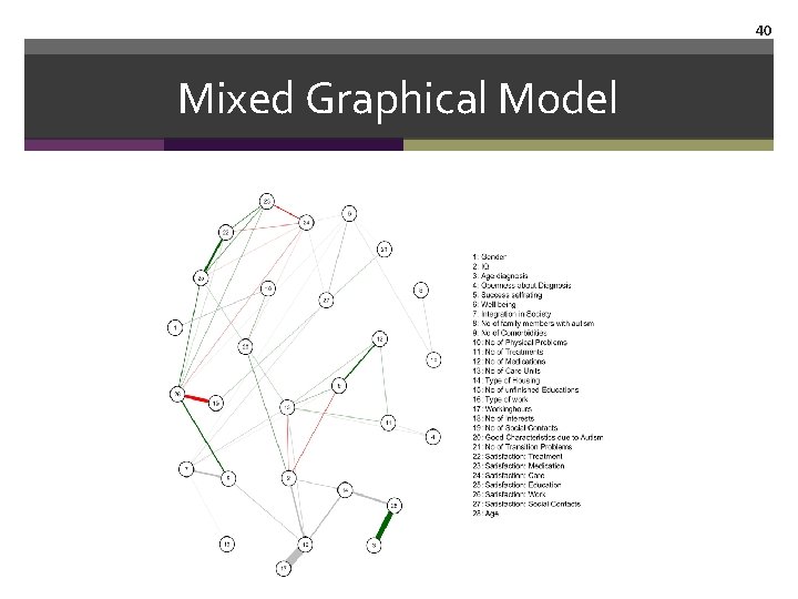
39 Mixed Graphical Model Estimate & visualize network fit. MGM <- mgmfit(Autism_data$data, Autism_data$type, Autism_data$lev, d=2) qgraph(fit. MGM$wadj, node. Names=Autism_data$colnames, layout='spring', edge. color=fit. MGM$edgecolor, legend. cex=. 3, vsize=3, legend. cex=1)

40 Mixed Graphical Model

Afternoon Session Overview Advanced methods • Part 1. Network Comparison Test • Part 2. Mixed Graphical Models • Part 3. Latent Variable Network Modeling Practical Session Any questions you have

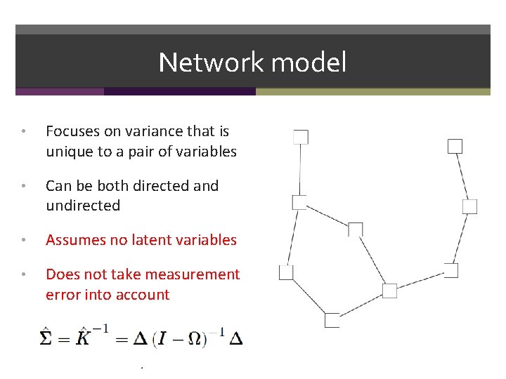
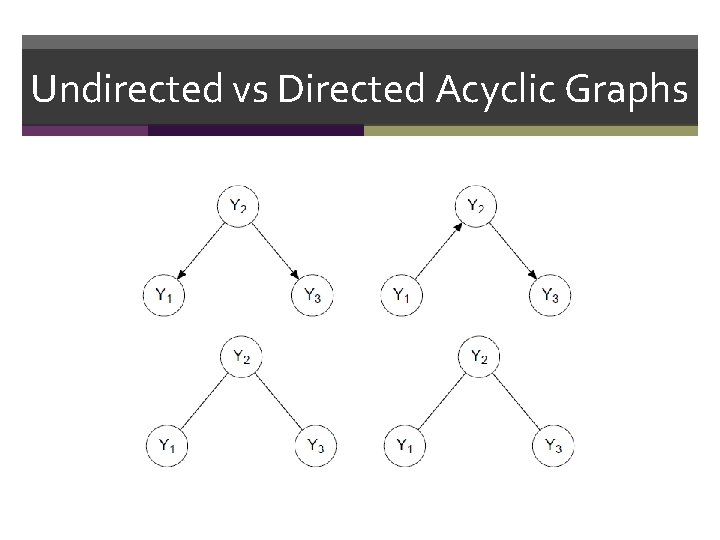
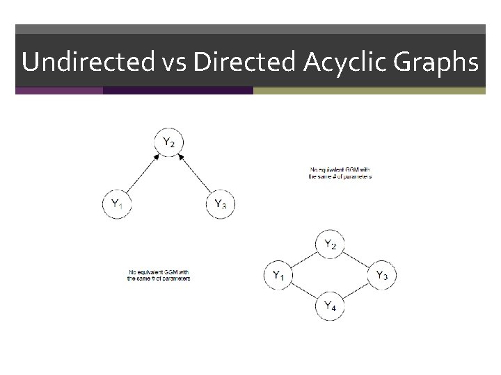
Network model • Focuses on variance that is unique to a pair of variables • Can be both directed and undirected • Assumes no latent variables • Does not take measurement error into account

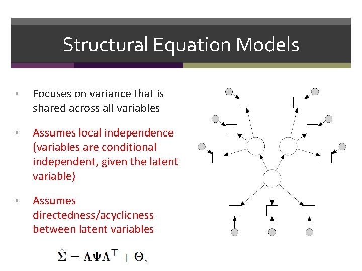
Structural Equation Models • Focuses on variance that is shared across all variables • Assumes local independence (variables are conditional independent, given the latent variable) • Assumes directedness/acyclicness between latent variables

Undirected vs Directed Acyclic Graphs

Undirected vs Directed Acyclic Graphs

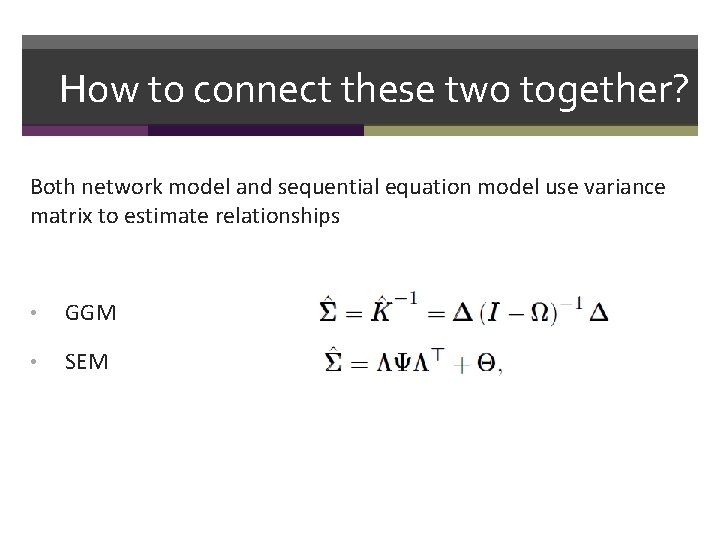
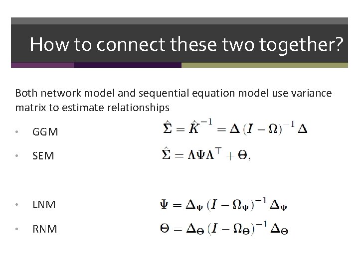
How to connect these two together? Both network model and sequential equation model use variance matrix to estimate relationships • GGM • SEM

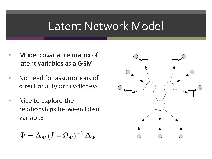
Latent Network Model • Model covariance matrix of latent variables as a GGM • No need for assumptions of directionality or acyclicness • Nice to explore the relationships between latent variables

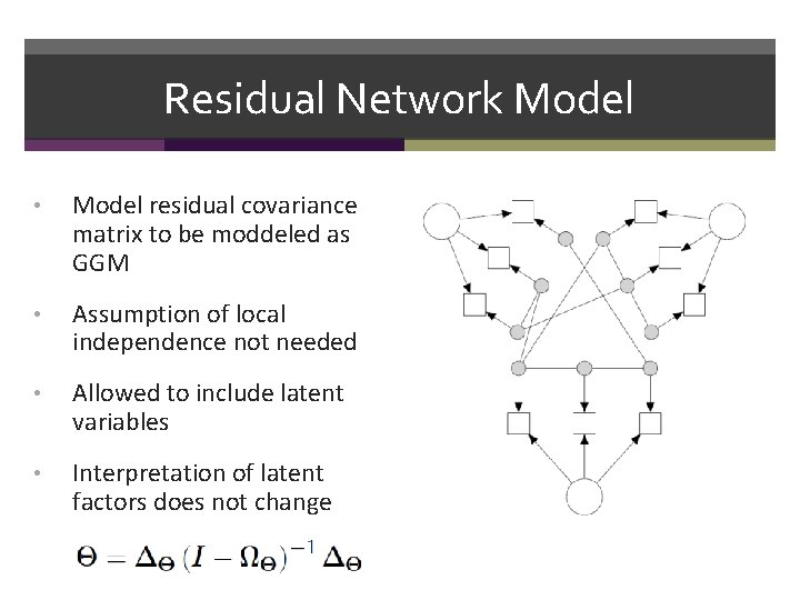
Residual Network Model • Model residual covariance matrix to be moddeled as GGM • Assumption of local independence not needed • Allowed to include latent variables • Interpretation of latent factors does not change

How to connect these two together? Both network model and sequential equation model use variance matrix to estimate relationships • GGM • SEM • LNM • RNM

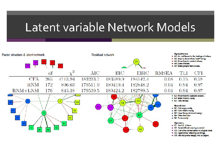
Latent Variable Network Models Both LNM and RNM, and the combination of the two… • Allow for confirmatory testing of network structures • Allow estimating the fit of a model • R package lvnet

Latent variable Network Models

52 Summary • Network Comparison Test (NCT) enables us to formally test whether two networks might be different • Mixed Graphical Models (MGM) can be used to estimate networks from mixed data. • Latent Variable Network Modeling provides us with a framework to combine latent variables with the network approach.

53 Break

Afternoon Session Overview Advanced methods • Part 1. Network Comparison Test • Part 2. Mixed Graphical Models • Part 3. Latent Variable Network Modeling Practical Session Any questions you have